
Introduction
Offshore industry development and operations require detailed characterisation of the shallow marine subsurface to identify geohazards and support safe engineering decisions. Applications include offshore wind farm development, shallow-hazard assessment for well planning, and site investigations for subsea infrastructure, pipelines and cables. These activities integrate geophysical, geotechnical, and geological information to identify geohazards and constrain ground conditions. Buried channels, boulders, shallow gas, and heterogeneous sedimentary units can pose risks to drilling, infrastructure installation and long-term asset integrity if they are not adequately characterised. High-resolution seismic imaging therefore plays an important role in resolving shallow structures at scales relevant to engineering and operational decisions.

Ultra high-resolution (UHR) refers to imaging that uses high-frequency seismic signals, including frequencies up to 1000 Hz, to resolve fine-scale shallow subsurface features. The high-frequency content of UHR imaging supports detailed imaging of the upper tens to hundreds of metres of the subsurface. Although two-dimensional (2D)-UHR data can provide excellent vertical detail, 2D acquisition and imaging cannot account for wave propagation associated with three-dimensional (3D) geological structures. Out-of-plane energy may therefore contribute to residual diffraction features and interpretation uncertainty, particularly around a rugose seabed and other complex shallow structures. These limitations motivate densely sampled 3D acquisition and imaging. 3D ultra high-resolution (3D-UHR) seismic surveys commonly use sparker sources and short-streamer configurations to map shallow stratigraphy, detect geohazards and guide geotechnical investigations (Kluesner et al., 2018; Lebedeva-Ivanova et al., 2018; Monrigal et al., 2017).
Recent developments in 3D-UHR marine acquisition systems aim to address these limitations by increasing both spatial and temporal sampling density. These systems are scaled-down versions of conventional towed-streamer 3D marine seismic acquisition optimised for shallow targets using high-frequency sources and closely spaced receiver arrays. In such configurations, sparker sources capable of emitting signals up to several kilohertz are typically deployed, while both sources and streamers are towed at very shallow depths (on the order of 0.5-2 m) to preserve high-frequency energy and enhance resolution. These datasets can resolve fine-scale subsurface features, provided the acquisition and imaging make full use of the bandwidth and spatial sampling. However, nominally dense CMP sampling does not necessarily translate into equivalent image resolution. Offset and azimuth coverage remain irregular within individual offset classes, while the source and receiver arrays introduce direction-dependent responses. The interaction between acquisition sampling, array responses and regularisation motivates the present numerical experiment.
In this study, we used numerical modelling to assess the recovery of metre-scale shallow targets for a representative wide-tow, four-source 3D-UHR marine acquisition geometry. Previous studies have highlighted the potential for metre-scale resolution under favourable acquisition and imaging conditions (Davies and Rietveld, 2020; Lebedeva-Ivanova et al., 2018). Our objective was to examine how acquisition sampling, finite-array responses and imaging workflow affect target separation and structural fidelity.
Synthetic seismic data with frequencies up to 1000 Hz were generated by acoustic finite-difference modelling using realistic source and receiver arrays. The velocity-density model included a variable-depth water bottom, rapidly vertical variations in velocity and density, 1116 diffractor blocks of prescribed sizes and separations and two additional complex spatial patterns. The synthetic data were processed through two alternative workflows: (1) a standard offset-class Kirchhoff pre-stack depth migration (PSDM) workflow and (2) a shot-domain time-lag full-waveform inversion (TLFWI) workflow (Zhang et al., 2020). The resulting images were compared with the known true model to evaluate and compare resolution and structural fidelity for the two workflows. A separate field-data example compared the 2D-UHR site-survey image with a PSDM image and a FWI image, both obtained from conventional 3D streamer data using frequencies up to approximately 200 Hz.
The field results provide complementary evidence of the benefits of FWI for shallow imaging, showing that it can improve structural detail relative to the tested PSDM workflow even when 3D-UHR data are unavailable.
Synthetic experiment
The synthetic experiment was designed to assess workflow-dependent lateral resolution for a representative 3D-UHR marine acquisition geometry.
1 Acquisition geometry
The modelled acquisition system consisted of a wide-tow 3D-UHR marine streamer configuration, illustrated in Figure 1. The setup included four dual-level sparker sources arranged in a wide-spread configuration, combined with ten parallel streamer cables. The streamers were separated by 8 m in the crossline direction, while receiver groups were spaced at 2 m intervals along each cable. Shot points were acquired with an inline spacing of 4 m, with an effective 1 m sampling achieved through flip–flop shooting.
This acquisition geometry had a nominal bin size of 1 × 1 m, providing the dense spatial sampling required to approach metre-scale lateral resolution. Dense spatial sampling in both inline and crossline directions was critical for adequately capturing high-wave number components of the wavefield. However, despite the nominal bin size, variations in source–receiver azimuths and offset distribution introduced non-uniform illumination, which may limit the effective resolution achievable in practice.
2 Source and receiver modelling
The seismic source used in the modelling was a dual-level sparker system, consisting of two rectangular 1.8 m × 0.75 m arrays of 400 sparker tips, each deployed at depths of approximately 0.6 m and 0.9 m, respectively mimicking a typical dual-level sparker geometry. The point source signature from each sparker tip was derived from measured sparker wavelets reported by Kluesner et al. (2018) and included the characteristic bubble oscillations associated with sparker sources (Figure 2). The wavelet used to construct the source response was ghost-free; source and receiver ghosts were introduced separately during forward modelling.
The usable frequency bandwidth of the source extended from approximately 50 Hz to 1000 Hz, providing the high-frequency content required for ultra-high-resolution imaging. In principle, such frequencies correspond to sub-metre vertical resolution and metre-scale lateral resolution, depending on the propagation velocity and illumination conditions.
Receiver arrays were modelled as 2 m-long hydrophone groups positioned at a depth of approximately 0.75 m. Hydrophone grouping improves signal-to-noise ratio through spatial averaging and filtering (Ursin, 1983) but also modifies the recorded signal. The group response depends on frequency and on the component of horizontal slowness along the streamer. For the example shown in Figure 3, grouping attenuated the higher-frequency content relative to a single hydrophone. This direction-dependent filtering can reduce the contribution of high-frequency energy to imaging and produces amplitude and waveform variations between source–receiver azimuths.
3 Model design
The subsurface model used for forward modelling is shown in Figure 4a. The model domain extends over 500 × 500 m laterally and 50 m in depth, with a uniform grid spacing of 0.5 m. This sampling ensured accurate numerical representation of wave propagation up to frequencies of 1000 Hz, supporting the targeted metre-scale resolution.
The water layer had a thickness between 15 m and 20 m with a smooth, S-shaped transition zone as shown in Figure 4b.
The background velocity and density models beneath the sea bottom were derived from a scaled well log from the Barents Sea (Figures 4c–d), with the corresponding reflectivity profile shown in Figure 4e.
On top of this background, reflectivity was introduced through a combination of discrete and continuous features (Figure 5). A total of 1116 diffractor blocks, implemented as density anomalies, were placed at a depth of approximately 25 m, with lateral sizes ranging from 0.5 m to 2 m and edge-to-edge spacing between 0.5 m and 2 m. The variation in block size tested target detectability, while the prescribed separations made it possible to distinguish neighbouring targets to be assessed (Figure 6a–b).
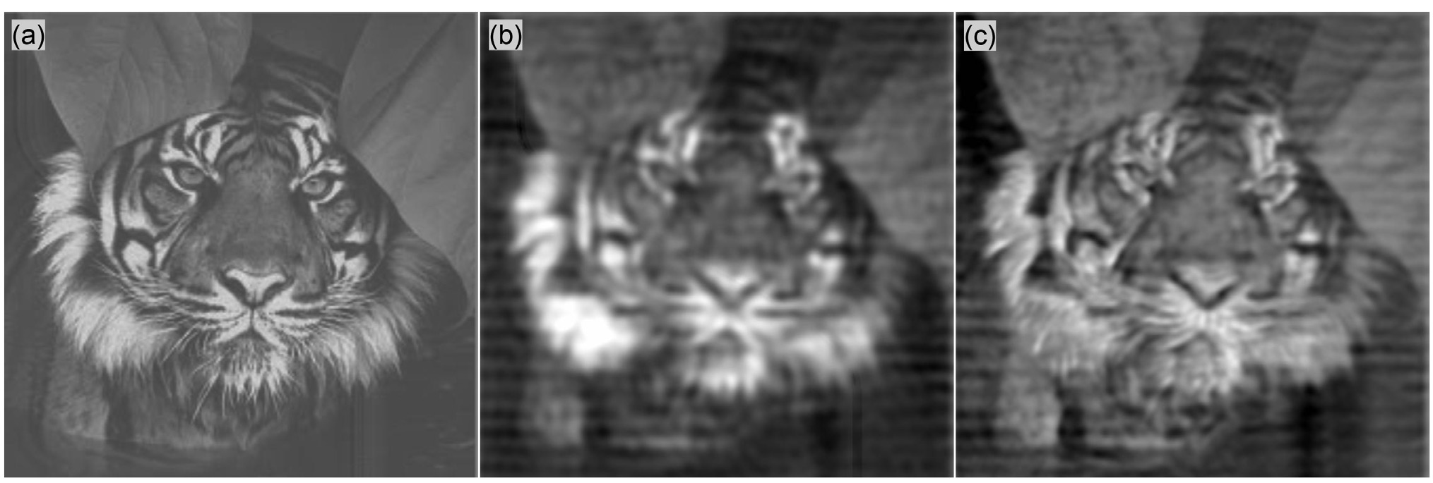
Additional targets were embedded at depths of approximately 30-45 m, including a spherical anomaly with a diameter of approximately 5 m and image-based ‘tiger’ and ‘satellite’ patterns. Figure 5 shows their vertical distribution, while Figure 6 shows the block targets and spherical anomaly in panels (a–b) and the ‘tiger’ and ‘satellite’ patterns in panels (c–d). These complex patterns provided controlled tests of structural fidelity over a wider range of orientations and spatial scales than the block targets.
4 Forward modelling
Synthetic seismic data were generated using an acoustic finite-difference scheme on a grid with 0.5 m spacing. The source wavelet contained frequencies between 50 and 1000 Hz. The modelled responses included primary reflections, diffractions and source and receiver ghosts. The synthetic traces are stored at a sampling interval of 0.5 ms.
The modelling setup was designed to isolate the effects of acquisition geometry and spatial sampling. Source and receiver ghosts were explicitly included using mirror sources and receivers at symmetric positions above the water surface, preserving the interference patterns associated with the shallow source and receiver depths.
The resulting synthetic shot gathers (Figure 7) show water-bottom reflections and diffraction responses from the embedded targets, with direct arrivals removed for clarity. Differences among the inner, middle, and outer streamers illustrate the influence of the source-receiver array response and geometry on the recorded wavefield.
Overall, the modelling framework represented an idealised acquisition scenario, characterised by noise-free data and perfect knowledge of the acquisition geometry. These assumptions allow the study to focus on the effects of acquisition design, wave propagation and imaging methodology on spatial resolution without additional field-data complexities.
3D-UHR PSDM and FWI processing and imaging
Two imaging workflows were applied to the synthetic observations: (1) an offset-class Kirchhoff PSDM workflow and (2) a shot-domain FWI workflow. Both used point-source/point-receiver representation rather than explicitly resolving the source/receiver arrays. The workflows are shown schematically in Figure 8.
The PSDM sequence followed a conventional workflow adapted to 3D-UHR data (Yilmaz, 2001). It comprised of six main steps: (1) deghosting and debubbling, (2) zero-phasing, (3) sorting into offset classes, (4) 4D interpolation and regularisation, (5) Kirchhoff PSDM of each offset class, and (6) angle muting and stacking.
Deghosting and debubbling were applied to reduce the acquisition-signature effects and prepare the data for zero-phasing and migration. Figure 9 illustrates the deghosting step, comparing the input, corrected data, and ghost-free reference. The corrected waveforms show improved agreement with the reference.
Following deghosting and debubbling, zero-phasing was applied to obtain a symmetric wavelet for migration. The data was then sorted into offset classes for Kirchhoff PSDM. Because of the wide-tow, multi-source acquisition geometry, however, the spatial and azimuthal sampling within individual offset classes was highly irregular. Figure 10 illustrates this irregularity for the nearest offset class within offset 4-12 m, in which only approximately 20% of the bins in the displayed area are populated and source-receiver azimuths vary substantially.
To obtain regularly sampled common-offset for Kirchhoff migration, 4D interpolation and regularisation were applied before migration to construct fully populated common-offset datasets. Figure 11 illustrates this step using the nearest offset class. The NMO-corrected inline, crossline and time-slice displays contained substantial sampling gaps, particularly in the crossline direction (Figures 11a–c). Migration of these sparse data produced a strong acquisition footprint and associated artefacts (Figure 11d).
After interpolation and regularisation, the data showed improved spatial continuity (Figures 11e–g). The corresponding migrated image contained less acquisition-related noise but lacked some details compared to the image obtained from the original sparse data (Figure 11h).
Figures 11, i–k, show an idealised, densely sampled 1 × 1 m zero-offset dataset, with the corresponding migration in Figure 11 (l). This experiment provided an idealised reference for reconstructing the target without spatial sampling gaps.
For the final PSDM image, Kirchhoff PSDM was applied independently to each regularised offset class using a smoothed version of the true velocity model. The migrated contributions were angle-muted and stacked over an incidence-angle range up to 45° to form the final PSDM image. The nearest-offset example in Figure 11 illustrates an intermediate processing step; the final image combines contributions from the retained offset classes and angles.
FWI, on the other hand, used the raw modelled shot gathers, without offset sorting, binning or pre-migration interpolation. The shot gathers contained the source and receiver array effects, ghosts and bubble as described above. In the inversion, however, the arrays were represented by point sources and receivers, with the vertical far-field signature of the source array used as the effective source wavelet. Starting from a heavily smoothed velocity model consistent with the velocity model used for migration, FWI iteratively updated the model by minimising the misfit between observed and simulated data (Tarantola, 1984; Virieux and Operto, 2009).
Velocity was the model parameter updated during inversion. Density was linked to velocity through Gardner’s law and was recalculated as the velocity model changed, rather than being inverted independently. A multiscale frequency-continuation strategy progressively incorporated frequencies from approximately 50 Hz to 1000 Hz. The final velocity model was converted into an FWI-derived image using Viridien’s proprietary FWI Imaging technology (Zhang et al., 2020; Huang et al., 2021). The PSDM and FWI-derived images were compared in terms of target separation and structural fidelity rather than direct amplitude equivalence.
Results and discussion
Figures 12 and 13 compare the reference targets with the final PSDM and FWI-derived images. The annotated block dimensions and separations in Figure 12 provide a spatial reference for assessing the resolution limits. For the blocks separated by 1 x 1 m (magenta colour), FWI is clearly able to separate them, whereas the individual blocks in the corresponding PSDM response are not distinguishable.
The lack of resolution of the Kirchhoff-based PSDM workflow was caused by three interacting aspects of the acquisition and processing.
First, spatial sampling within individual offset classes was incomplete. In the nearest offset for instance, only approximately 20% of the bins were populated, with strongly varying source–receiver azimuths (Figure 10). A nominal 1 × 1 m midpoint grid therefore did not imply complete sampling of the wavefield within each offset class. In the Kirchhoff-based PSDM workflow, the empty bins were interpolated in the pre-migration regularisation to avoid PSDM acquisition footprints.
Second, interpolation and regularisation introduced a trade-off between acquisition-footprint suppression and preservation of fine detail in the final image. In Figure 11 (e-h), improved data continuity was accompanied by a smeared migrated image, particularly across the more sparsely sampled crossline direction. This behaviour is consistent with incomplete recovery of the high-spatial-wavenumber content needed to reconstruct closely spaced model blocks and diffraction patterns.
Third, azimuth-dependent receiver-group responses add variability between traces within an offset class. Figure 14 compares traces for similar offsets but different source–receiver azimuths. Traces like these will typically be present in a near-offset class input to regularisation. The selected point-receiver responses showed relatively small amplitude differences, whereas the array-modulated responses varied more strongly with azimuth. This additional variability complicated the reconstruction of sparsely sampled offset-azimuth data.
These differences are caused by variations in incidence wave directions to the receivers. When propagation direction is nearly parallel to the streamer, the component of horizontal slowness along the receiver group is larger, producing greater time delays across the group and stronger frequency-dependent filtering. When propagation is more perpendicular to the streamer, the along-group time differences are smaller, and the group response is more uniform over frequencies. Consequently, the recorded waveform depends on frequency and source–receiver azimuth. Reflector depth and dip can also influence the response by changing the incidence direction at the receivers.
Together, Figures 10, 11 and 14 illustrate how incomplete offset-class sampling and directional array responses can complicate pre-migration regularisation. In the tested PSDM workflow, the reduction in acquisition footprint was accompanied by a loss of fine spatial detail and a 1 m resolution was not achieved.
Unlike the tested PSDM workflow, FWI did not require offset-class regularisation; it evaluated the data misfit at the acquisition shot and receiver coordinates. Although the recoverable spatial wavenumbers remained constrained by illumination, acquisition responses and inversion assumptions, the 1 m resolution was clearly achieved as can be seen in Figure 12.
The synthetic experiment represents favourable conditions: the observations are noise-free, the acquisition geometry is exactly known, the sea surface is flat and horizontal, and both workflows use a smoothed background derived from the true model. In addition, the prescribed velocity-density relationship used in FWI may differ locally from the real density model. Therefore, the key question remains whether the observed advantage of FWI persists in real field data where noise, positioning uncertainties, wavelet variability and geological complexity are unavoidable.
To address this question, a field-data example provides a complementary perspective on the application of FWI to shallow imaging with 3D seismic data under practical acquisition conditions.
Field-data demonstration
Two examples are from the Barents Sea with water depths of approximately 400 m, where rugose seabed topography and shallow gas pockets are key challenges for seismic imaging (Dinh et al., 2024). Data used for PSDM and high-resolution FWI imaging in this section came from a source-over-spread survey with six separated sources and sixteen 8 km-long cables. Although this configuration is less densely sampled than the synthetic 3D-UHR acquisition, it is one of the densest industrial-scale seismic acquisitions currently available, which provides dense spatial sampling and full-azimuth coverage at near offsets. Hence, it can be utilised as a test of whether the conclusions drawn from the synthetic study remain valid under practical acquisition conditions.
In addition to the source-over-spread dataset, a site survey consisting of 2D-UHR seismic was available over the study area. These datasets were used as independent references to compare shallow imaging performance, seabed morphology and the interpretability of the PSDM and FWI results, since 2D-UHR data is a common reference for near-surface studies undertaken for well planning.
Example 1: Complex seabed structure
As shown in Figure 15, conventional 3D PSDM imaging struggles to resolve the rough water bottom densely etched with relic iceberg ploughmarks. In addition, key shallow features are missing due to limited illumination. On the other hand, the 100 Hz FWI image provides significant increased vertical and spatial resolution, resulting in detailed seabed and reliable subsurface structure. It also resolves small-scale low-impedance features, commonly associated with gas pockets and faults – that are not clearly visible in the PSDM.
Example 2: Shallow geology resolution
This example examines a shallow interval in an area of complex overburden geology and numerous interpreted shallow gas pockets. Figure 16 compares the images over an interval extending approximately 100 ms below the seabed. The 2D-UHR image retains fine vertical detail, but its limited azimuthal coverage and recording aperture leave bowtie effects and shallow diffractions unresolved (red arrows). The conventional PSDM image shows a more clearly defined seabed and fewer visible artefacts, but at this scale lacks the spatial detail required to characterise shallow geology. On the other hand, 200 Hz FWI at this location, while limited by the Nyquist frequency with this 2 ms sampled data, shows a sharper seabed response (purple arrow) and additional intra-sedimentary features, including finer-scale gas pockets that are not clearly resolved in the PSDM image (green arrows).
Conclusion
The synthetic comparison showed that nominal 1 × 1 m midpoint binning and a source signal up to 1000 Hz did not, by themselves, guarantee equivalent lateral image resolution. In the offset-class Kirchhoff PSDM workflow, sparse lateral sampling and direction-dependent acquisition array responses complicated pre-migration regularisation, leading to a loss of fine target detail.
Applied to the same source/receiver array-generated modelled data, FWI produced improved target separation and structural fidelity and demonstrated a lateral resolution down to 1 m.
The field example agreed with the conclusion of the synthetic study: given a conventional (non-UHR, but still dense) 3D data set, an FWI approach provides better resolution than a standard Kirchhoff-based approach.
Whether using an idealised, synthetic 3D UHR survey or a real dense 3D source-over-spread survey, the maximum achievable resolution ultimately depends on how effectively the recorded wavefield is utilised. FWI has been shown on both synthetic and field data to better recover the Earth’s reflectivity, improving spatial resolution over conventional migration from the same data. It has therefore shown that the imaging technology can at least partly compensate for sparser acquisition setups and improve near-surface resolution. This suggests future efforts aimed at achieving metre-scale seismic imaging should not focus exclusively on increasingly dense acquisition designs but consider FWI as the method of choice for maximising resolution from the data.
Acknowledgment
The authors would like to thank Viridien for permission to publish this work and acknowledge colleagues for helpful discussions and contributions to the study. We would also like to thank Vår Energi and partner OMV, Viridien Earth Data and TGS for permission to use and present the data. The scientific content, interpretation of results, and conclusions were developed and verified by the authors, who take full responsibility for the final manuscript.
References
- Davies, D. and Rietveld, W. [2020] The journey to 1 m resolution at Clair – lessons from acquisition and processing. Second EAGE Marine Acquisition Workshop, Extended Abstracts. DOI: 10.3997/2214-4609.202034003.
- Dinh, H., Latter, T., Townsend, M., Grinde, N., Hogden, S., Robb, N., Aksland, M. and Bertrand, A. [2024] High-frequency FWI imaging: repurposing seismic data for imaging shallow hazards. First Break, 42(8), 55-63. DOI: 10.3997/1365-2397.fb2024064.
- Huang, R., Zhang, Z., Wu, Z., Wei, Z., Mei, J. and Wang, P. [2021] Full-waveform inversion for full-wavefield imaging: Decades in the making. The Leading Edge, 40(5), 324-334. DOI: 10.1190/tle40050324.1.
- Kluesner, J.W., Brothers, D.S., Hart, P.E., Miller, N.C. and Hatcher, G.A. [2018] Practical approaches to maximizing the resolution of sparker seismic reflection data. Marine Geophysical Research, 40(3), 279-301. DOI: 10.1007/s11001-018-9367-2.
- Lebedeva-Ivanova, N., Polteau, S., Bellwald, B., Planke, S., Berndt, C. and Stokke, H.H. [2018] Toward one-meter resolution in 3D seismic. The Leading Edge, 37(11), 818-828. DOI: 10.1190/tle37110818.1.
- Monrigal, O., de Jong, I. and Duarte, H. [2017] An ultra-high-resolution 3D marine seismic system for detailed site investigation. Near Surface Geophysics, 15(4), 335-345. DOI: 10.3997/1873-0604.2017025.
- Tarantola, A. [1984] Inversion of seismic reflection data in the acoustic approximation. Geophysics, 49, 1259-1266.
- Ursin, B. [1983] Spatial filtering of marine seismic data. Geophysics, 48(12), 1611-1630. DOI: 10.1190/1.1441443.
- Virieux, J. and Operto, S. [2009] An overview of full-waveform inversion in exploration geophysics. Geophysics, 74(6), WCC1–WCC26. DOI: 10.1190/1.3238367.
- Yilmaz, Ö. [2001] Seismic Data Analysis: Processing, Inversion, and Interpretation of Seismic Data. Society of Exploration Geophysicists.
- Zhang, Z., Wu, Z., Wei, Z., Mei, J., Huang, R. and Wang, P. [2020] FWI Imaging: Full-wavefield imaging through full-waveform inversion. SEG Technical Program, Expanded Abstracts, 656-660. DOI: 10.1190/segam2020-3427858.1

