Towards more cost-efficient and higher-quality sparse nodal surveys

Introduction

Ocean Bottom Node (OBN) surveys took off in the E&P industry in support of deep-water development and near-field exploration (Beaudoin et al., 2007; Beal et al., 2014). For such surveys, node spacing ranges between 200 and 400 m, and a source sampling of 50 by 50 m has become the norm. The first OBN survey for exploration was acquired by BHP in 2018 (Lin et al., 2021). It was followed quickly thereafter by the first multi-client OBN survey for exploration, the Amendment 1 survey (Roende et al., 2020), which was acquired in 2019. To cover areas relevant for exploration, both surveys deployed nodes on a 1 by 1 km grid. The shot carpets surrounded the nodal ones by halos of 15 and 20 km, respectively.

Data like this naturally have very large offsets, which allow full waveform inversion (FWI) to update the velocity model down to the sedimentary basement and into the lower crust of the Earth. It is fair to say that sparse nodal surveys for exploration have since revolutionised subsalt imaging (Vigh et al., 2023; Merritt et al., 2024; De Marco Centeno et al., 2026).

The main difference between the first two sparse nodal surveys was the shot density. The BHP survey used a fairly sparse shot grid of 200 by 400 m, which leads to data most suitable for FWI-based velocity model building. The Amendment 1 survey used a much denser shot grid of 50 by 100 m, allowing for higher resolution imaging. With a source area of 8000 km², there were approximately 1.6 million shot points in the Amendment 1 survey. Shooting such a large number of shot points was achieved by using three source vessels, each towing two airgun arrays separated by 100 m in the crossline direction and shooting in a flip-flip manner with time dithers in the order of 1 s. Later sparse nodal surveys for exploration used two source vessels with three source arrays separated by 100 m in the crossline direction, shooting dithered flip-flop-flap style, or even 4 sources firing dithered flip-flop-flap-flup style.

Vigh et al. (2021) illustrate the amount of simultaneous source interference in the data acquired with two triple source vessels. This interference consists mostly of strong direct arrivals on top of weaker refractions and reflections, which need to be attenuated before application of FWI and Reverse Time Migration (RTM) through deblending (Abma and Foster, 2020). The success of FWI on sparse nodal surveys shows that this strategy is effective. It is, however, unknown to what extent the convergence of FWI is affected by remnant interference after deblending and/ or by damaged diving/refracted wave signal, especially at very low frequencies, which help in avoiding cycle skipping.

Apparition encoding (Andersson et al., 2017; Amundsen et al., 2018) is a different way of simultaneous shooting. Rather than applying large (~ 1 s) random dithers in the firing times, shots are fired with small, deterministic variations in firing times. These variations are typically smaller than 200 ms, so strong direct arrivals are kept together, as are weak reflections and refractions. This so-called strong-on-strong, weak-on-weak property facilitates the decoding process. On top of this, very low frequencies stack up in phase for such small relative delays, while ambient noise is measured only once during a salvo of encoded shots. Apparition encoded shooting therefore has a natural SNR ratio improvement for very low frequencies.

In this paper, we compare conventional dithered shooting against Apparition encoded shooting based on a field test during a conventional sparse nodal survey conducted in 2025. The comparison is between dithered sequential quad-source data and encoded hexa-source data. The latter can obviously be more cost-efficient than the former. After deblending and decoding, we observe a significant uplift in SNR on the decoded data over the full bandwidth, which is especially impressive at very low frequencies. This has a marked effect on low-frequency FWI results. While the difference in SNR may have partially been caused by differences in sea state during acquisition, the results suggest that encoded shooting may also enable higher quality sparse nodal surveys for exploration.

Description of the field test

The field test of hexa-source Apparition encoded shooting was conducted during the Amendment West 1 (AW1) multi-client sparse nodal survey, which was acquired in 2025 and 2026. We will refer to this multi-client survey as the production survey. Both production and test data were shot with the Gemini-enhanced frequency source (Udengaard et al., 2023), which has strong low-frequency content. The production survey used two quad-source vessels to keep source and receiver efforts in balance. The field test was executed with a single hexa-source vessel.

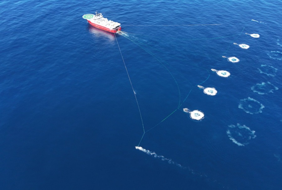
The Apparition test comprised six hexa-source sail lines. The sources were 60 m apart in the crossline direction, encoded salvos of 6 shots were fired at 60 m inline increments. Figure 1 shows such a salvo. Because of limitations in compressor capacity, we had to lower the firing pressure to 1500 psi during the test. The sail lines were roughly 60 km long. The test data therefore consists of a narrow source swath of 2.1 by 60 km sampled on a regular 60 by 60 m grid.

The production data were shot with four Gemini sources firing dithered flip-flap-flop-flup style on a staggered 100 by 50 m grid. Firing pressure was 2000 psi. Nodes were placed on a 1200 by 1200 m grid. For the comparison in this paper, we have extracted six sail lines of production data, which covered approximately the same area as the test data (2.3 by 60 km). To compare these data while the production survey was still ongoing, 19 extra nodes were co-located with production nodes along a sail line and retrieved ahead of the production nodes.

Table 1 summarises the key acquisition parameters for production and test surveys for easy reference.

Figure 2 shows a comparison of a nodal record of production and test data after a 0.2 Hz low-cut filter to remove low-frequency swell. This figure nicely visualises the key difference between dithered quad-source shooting and encoded hexa-source shooting. In the first case, strong events overlay weaker ones; in the second, strong events are kept together. This strong-on-strong, weak-on-weak property holds until the next salvo, 32.4 s later at a vessel speed of 3.6 knots (1.9 m/s). The encoded data have 6 events on top of each other with encoding delays, giving them a ‘fuzzy’ character. Decoding will separate this record into 6 single-source records with sharp events. Deblending of the dithered data will attenuate the strong-on-weak interference.

Low frequency considerations

Firing six shots with small delays with an array of Gemini sources 60 m separated in the crossline direction approximately leads to a six-fold increase in signal strength at very low frequencies compared to firing a single Gemini source, because the individual source contributions sum up approximately in phase. The signal amplification is frequency-dependent, of course, and in fact, it also weakly depends on the horizontal offset between the centre of gravity of the source array and the node.

To get an impression of the signal amplification as a function of frequency and horizontal offset, we consider a node at a depth of 1000 m, and a source array positioned at two locations, with the centre of gravity of the array 0 and 30 km away from the node in the horizontal direction, respectively. We assume that the individual guns in the source array are distributed along a line orthogonal to the horizontal line connecting the centre of gravity of the array and the horizontal location of the node. We will write $r_i$ for the distance between gun $i$, $(i=1,2,\cdots ,6)$, and the node, and for $r_0$ the distance between the centre of gravity of the source array and the node. Assuming point source behaviour for the individual guns, and ignoring the source signature and source ghost, the arrival of an encoded salvo takes the form

$$d(t)=\sum _{i=1}^6\frac{1}{4\pi r_i}\delta \left(t-\frac{r_i}{c_w}-\Delta t_i\right).$$

Here $c_w=1500m/s$ is the sound speed in water and $\Delta t_i,i=1,\cdots ,6$, are the encoding delays. The Fourier transform of this expression takes the form

$$\hat{d}(f)=\sum _{i=1}^6\frac{1}{4\pi r_i}{e}^{2\pi if\left(\frac{r_i}{c_w}+\Delta t_i\right)}.$$

In order to quantify the amplitude amplification relative to a single source, we now divide by the Fourier transform of data due to a single shot at the centre of gravity of the array and take its absolute value. This leads to

$$A(f)=\left|\sum _{i=1}^6\frac{r_0}{r_i}{e}^{2\pi if\left(\frac{r_i-r_0}{c_w}+\Delta t_i\right)}\right|.$$

The amplification curves as a function of frequency for source arrays at offsets 0 and 30 km fired with the same encoding delays of [0.092, 0.104, 0.064, 0.028, 0.128, 0.024] s. are shown in Figure 3. We have also calculated the amplification factor for a source array at 30 km offset with different encoding delays of [-0.096, -0.14, -0.172, -0.08, -0.112, -0.128] s. Both these encoding delays were taken arbitrarily from the encoding table used in the field. We note that for low frequencies the signal gets amplified by approximately 6, with small variation due to location of the source array or encoding delays. It therefore holds more or less uniformly for the direct arrival going into the earth, and also for the backscattered wavefield.

Ambient noise is measured only once during an encoded salvo of such a short duration, so the SNR in encoded data also goes up by a factor of approximately 6 at low frequencies compared to shooting a single source. For these low frequencies, one can treat the encoded data as ‘super’ shots, which could be used directly in low-frequency Reverse Time Migration (RTM) and FWI calculations, that is, without even decoding them. Both these algorithms stack over shots in calculating the contribution of a node to an image or a gradient of an objective function with respect to velocity. Assuming uncorrelated (between salvos) random noise, the SNR thereby increases by the square root of the number of terms in the stacks. If one stacks super shots, there will be 6 times fewer terms, but each term has an SNR 6 times higher than for normal shots. The net effect is an improvement of low-frequency SNR by a factor $\sqrt{6}$ in the stacks.

If we do decode the data and use these in a stack, the SNR improvement compared to stacking single-source data should be the same, of course. The number of terms in the stacks over decoded and single-source data is the same then, so there is no relative change in SNR due to the stack in this case. This illustrates that we should expect a $\sqrt{6}$ improvement of SNR on decoded data before stacking.

In conclusion, on encoded data low-frequency SNR improves by a factor of 6 because the signal sums up coherently and only one copy of the ambient noise is measured. On decoded data, low-frequency SNR is expected to improve by a factor $\sqrt{6}$.

Compressor capacity of the source vessel only allowed for a firing pressure of 1500 psi for the hexa-source test lines, as opposed to the standard 2000 psi during the quad source production lines. Since the spectral output below the resonance frequency of the airgun scales as $p^{4/3}{f}^2$ (Baeten et al., 2021), the SNR of the encoded data should be reduced by a factor of ~0.7 for these frequencies.

On theoretical grounds, the difference in source sampling between production and test data should lead to a factor of $\sqrt{100\times 50}/60\approx 1.2$ improvement of SNR in RTM images or FWI gradients based on decoded data compared to production data. Below the resonance frequency of the airgun, the net SNR improvement in RTM images or FWI gradients should therefore be $0.7\times 1.2\times \sqrt{6}\approx 2$, showing that there is ample room to go to wider hexa-source tows, while retaining good SNR. In fact, the only reason for not towing wider in the test was the absence of suitable in-water equipment.

Apart from these considerations, the inverse problems solved in deblending and decoding deal with noise in different manners, which can only be compared by analysing data and image domain results based on the field test. This will be done in the next two sections.

Data domain comparisons

The six quad-source dithered sail lines and the six hexa-source Apparition encoded sail lines were deblended and decoded, respectively. The results in various frequency bands are shown in Figure 4.

The SNR on the Apparition decoded data is clearly superior, both for the low frequencies and over the full bandwidth. The former can be partially understood by the considerations in the previous section. The latter suggests that ambient noise rejection in the inverse problem for decoding is more effective than in the inverse problem for deblending. It should be mentioned, however, that the background noise level at low frequencies was higher during the shooting of the production lines going into the test than during the Apparition test due to the sea state, which may also partially explain the difference in SNR between deblending and decoding in the low frequency bands.

Image domain comparisons

The deblended quad source production data and the decoded hexa-source data, as recorded by the 19 test nodes at 1200 m spacing, were subsequently imaged by RTM. We used an existing velocity model, which has been derived from towed-streamer WAZ data acquired in the survey area. Figure 5 shows a comparison of 12 Hz RTM images. Minimal preprocessing in the form of zero phasing and debubble has been applied to both data sets. The image of the deblended production data is on the left; the image of the decoded Apparition data is on the right. The image of the full towed streamer WAZ data is shown in the middle as a reference. It is obvious that the combination of a single line of 19 nodes spaced at 1200 m and a 2.3 km (for the deblended data) or 2.1 km (for the decoded data) by 60 km source swath has quite limited illumination properties. The towed-streamer WAZ image has totally different illumination properties, so it only serves as a guide for what the subsurface looks like.

The main conclusion from this comparison is that the image of the decoded Apparition data is on par with the image of the deblended production data.

We next examined whether the low-frequency data-quality differences observed in Figure 4 translate into differences in FWI results. To this end, we have taken a velocity model derived from a 1.8 Hz elastic FWI on the full production data. This is shown in Figure 6a. We have applied a 3% velocity perturbation to this model, which is shown in Figure 6b. Subsequently, we have calculated FWI sensitivity kernels in the perturbed velocity model for a single node and offsets in the 15-20 km range on data low passed by a filter with corner frequencies 0.6 and 1.2 Hz, the frequency band which we typically use to start off FWI on deep water sparse nodal surveys. These kernels are visualised in Figure 6c for the deblended quad-source data and in Figure 6d for the decoded hexa-source data. We have also run a full FWI update for deblended data (Figure 6e) and for decoded data (Figure 6f) in the same frequency band.

It is clear that the sensitivity kernels of the decoded data are more spatially coherent than the ones based on deblended data. Also, the FWI result based on the decoded data is in closer qualitative agreement with the actual velocity perturbation shown in Figure 6b than the one based on deblended data. Given the difference in low-frequency SNR visualised in the bottom row of Figure 4, this should not come as a surprise.

In practice, we have seen good results with FWI when using all nodes and all shots in a quad-Gemini dithered survey (Xing et al., 2026). As mentioned before, the background noise level at low frequencies was higher during the acquisition of the production sail lines used in the test than during the acquisition of the Apparition test lines. Using data collected in a full survey, one would add many more sail lines and these effects may partially average out. It is therefore possible that the FWI results for full survey data would look more comparable. This said, the low-frequency FWI results based on decoded data are very encouraging and may lead to faster convergence of FWI, more accurate FWI results and/or the possibility of starting from poorer initial models, for example models with large errors in salt geometry.

Conclusions and outlook

In this small-scale test, hexa-source encoded Apparition shooting at 1500 psi led to better SNR in the data domain and a better velocity update for low-frequency FWI than dithered quad-source data at 2000 psi, while being on par for RTM imaging. This low-frequency SNR difference can be attributed to several factors. First, we have argued that Apparition encoded shooting has an inherent SNR improvement due to low-frequency signals stacking up in phase and noise being measured only once during an encoded salvo. Second, deblending and decoding deal with noise in a different manner. Finally, there were differences in noise conditions during the acquisition of the production sail lines going into the test and the acquisition of the encoded sail lines.

The 6 sources in the test were separated by 60 m in the crossline direction, leading to a sail line spacing of 300 m, which is smaller than the 400 m for the production survey, which used 4 sources at 100 m crossline spacing. As mentioned, the reason for not towing wider during the test was the absence of suitable in-water equipment. Towing the 6 sources at 100 m crossline spacing would lead to 600 m sail line spacing and would be more cost-efficient, as the survey could then have been done with only a single source vessel.

The FWI results based on decoded data may lead to faster convergence of FWI, more accurate FWI results and/or the possibility of starting from poorer initial models, for example models with large errors in salt geometry. All these hypotheses need to be tested based on a full-scale survey with encoded data.

References

• Abma, R. and Foster, M.S. [2020] Simultaneous source seismic acquisition. SEG Geophysical Development Series, 18.
• Amundsen, L., Andersson, F., van Manen, D-J., Robertsson, J.O.A. and Eggenberger, K. [2018] Multisource encoding and decoding using the signal apparition technique. Geophysics, 83(1), V49-V59.
• Andersson, F., Robertsson, J.O.A., van Manen, D. J., Wittsten, J., Eggenberger, K. and Amundsen, L. [2017] Express Letters: Flawless diamond separation in simultaneous source acquisition by seismic apparition. Geophysical Journal International, 209(3), 1735-1739.
• Baeten, G., Hunt, K., Kuvshinov, B., Macintyre, H., McDonald, M., Nolan, B., Rambaran, V. and ten Kroode, F. [2021] Cheaper and Better Long Offset Nodal Surveys Based on Low-Frequency Enhanced Sources. 82^nd EAGE Annual Conference & Exhibition, Extended Abstracts.
• De Marco Centeno, R., Ji, S., Yang, Z., Flower, R., Wray, B., Zhu, H., Ronen, S. and Wentzler, P. [2026] Advancing subsalt imaging in the US Gulf: Operational and technical innovations in seismic data acquisition from the Laconia sparse OBN program. The Leading Edge, 45(2), 81-90.
• Lin, F., Ren, D., Mei, J., Xue Z., Blanch, J., Cahoj, M., Jarvis, J. and Kostin, A. [2021] Exploring the full potential of a sparse nodes survey in the Western Gulf of Mexico. First International Meeting for Applied Geoscience and Energy, Expanded Abstracts, 51-55.
• Merritt, M., Baeten, G., Rambaran, V., Godfrey, K., Bianchini, K., Brothers, T., Chelminski, F., Hao, A., Gao, H., Su, Y. and Wei, Z. [2024] Revealing the subsalt in garden banks with a sparsely-shot TPS OBN and FWI. Fourth International Meeting for Applied Geoscience and Energy, Expanded Abstracts, 958-962.
• Udengaard, C., Brookes, D. and Flores, H. [2023] Gemini: a fully operational broadband source for model building and imaging. Third International Meeting for Applied Geoscience & Energy, Expanded Abstracts.
• Vigh, D., Cheng, X., Lyons, K., Seymour, N., Kocel, K. and Pan, Z. [2021] Sparse-node regional study from acquisition to imaging. First International Meeting for Applied Geoscience & Energy, Expanded Abstracts, 722-726.
• Vigh, D., Cheng, X., Xu, J. and Jiao, K. [2023] Forge ahead in acquisition and model building via full-waveform inversion: Gulf of Mexico case study. Geophysics, 88(5), B285-B295.
• Xing H., Huang, R., Yuan, Z., Abdelaziz, K., Udengaard, C, Castelan A. and Hegazy, M. [2026] Gemini-Enabled Sub-Hertz Elastic FWI for Robust Subsalt Velocity Model Building. Fifth International Meeting for Applied Geoscience & Energy, Expanded Abstracts.