
Indirect inversion schemes create synthetic data with a forward modelling engine and compare them to the observed field data. The inversion then iterates so as to minimise the difference between the observed and modelled data: ideally, we perform the modelling with as many physical parameters as possible to create realistic synthetic data. However, in general we do not update (invert for) all the parameters we forward modelled with. In a previous tutorial, I outlined the mechanics of an acoustic time-domain waveform inversion algorithm employing a steepest descent method to estimate velocity. In this tutorial, I will review the current state of the art expanding the coverage to multi-parameter waveform inversion with an emphasis on anisotropy and reflectivity, to assess what is currently being inverted for and the degree to which inverted parameters are coupled. In addition, I will briefly mention the extension to the elastic case, and here it should be noted that current elastic implementations of full waveform inversion are still for the most-part working with P-wave data only, hence, in these situations we are not inverting against directly measured shear or density information, but rather relying on P-wave Amplitude Variation with Angle (AVA) behaviour to unpick elastic parameters.
Introduction
In the context of parameter estimation, inversion is a procedure wherein we try to estimate the physical parameters associated with a process via analysis of observations made on the outcomes of this process. Algorithmically, direct inversion involves solving a set of (usually) linear equations, typically with more equations than unknowns, in order to determine the unknown parameters, However, industrially, we tend to rely on indirect inversion schemes. With indirect inversion, we take an initial guess of the system’s parameters and then using some theoretical formulation of the system’s behaviour, we perform a forward modelling exercise to create synthetic data. In the geophysical context, these system parameters relate to the elastic properties of the Earth (velocity, anisotropy, density, attenuation 1/Q, etc) and the theoretical formulation refers to the type of wave equation we use for the forward modelling (e.g. constant density acoustic, variable density acoustic, visco (Q) acoustic, fully elastic, etc). In addition, in order to implement the modelling with our chosen theoretical formulation we also have to employ a numerical method on the computer (e.g. phase shift, finite difference (FD), finite element (FE), spectral element (SE), etc.). Full Waveform Inversion (FWI) is also employed in other fields, such as in global seismology to determine whole-Earth structure (e.g. Tromp, 2020), borehole cross-hole analysis (e.g. Pratt and Shipp 1999), medical imaging (e.g. Guasch et al., 2020), and metallurgy (e.g. Aktharuzzaman 2024).

The problem now becomes one of minimising the difference between the observed field data and the numerically modelled synthetic data, and here we have an enormous field of study in itself (e.g. Jackson 1972; Menke 1989). This is where the notion of a ‘norm’, ‘objective function’ or ‘cost function’ comes in; we need to minimise something related to the differences we observe, but here there are many very different options. We could for example minimise the difference just in arrival times between the observed and modelled events (in other words, only using the kinematics of the problem), or we could minimise the difference in amplitudes of the events (i.e. the dynamics of the problem), or just differences in the phase spectra, or perhaps a combination of both arrival time and amplitude differences, such as in the optimal transport (OT) method (otherwise known as the earth-movers problem, or the Wasserstein norm, e.g. Métivier et al., 2016a, 2016b).
The methods with the highest resolution are most likely to be ones where we use the amplitude information in the waveforms, which inherently also include all arrival time and phase information. However, these may also be the most error-prone methods, as we might not have ‘good enough’ amplitude and phase behaviour in the forward modelling, and more importantly, if the initial model is inaccurate, the procedure can fail. In general, forward modelling always tends to overestimate the amplitude of the synthetic waveforms. This is because we tend to simplify the forward modelling equations, and thereby ignore some of the underlying physical processes that take energy from the P-wave reflection events. For example, if we ignore attenuation effects in the modelling, the modelled data will have higher amplitudes than the real-Earth attenuated data amplitudes. Likewise, if we ignore elastic mode-conversion at the interfaces in the Earth, then we will not have accounted for energy that is transferred from the compressional-wavefield into the shear-wavefield, etc. The consequence of these various aspects is that the inversion tends to get ‘stuck’ in a local minimum, providing a nice-looking, detailed, but incorrect model (often as a result of cycle-skipping: i.e. aligning the wrong peaks and troughs of the modelled and observed data).
Consequently, most practitioners prefer alternative norms (at least in the initial stages of iterating the inversion), namely ones that are less prone to cycle skipping, and an overall strategic approach to the problem might thus be to start with some cycle-skip-avoiding norm such as adaptive (Warner and Guasch, 2014a, 2014b; 2015; 2016), adjustive time-lag (Jiao et al., 2015; Vigh et al., 2017; Wang et al., 2018), dynamic warping/matching (Mao et al., 2020; Huang et al., 2023), or phase-only (Maharramov et al., 2017; Schuster, 2017), and later (once the model is acceptably refined) move on to an optimal transport (Métivier et al., 2016a, 2016b; Yang and Engquist, 2018) or Least Squares (LS) amplitude norm for final fine-tuning.
In this tutorial, I will outline the move away from inverting only for isotropic velocity (with a constant density assumption) to inverting for both reflectivity and anisotropic parameters, with the emphasis being placed on the interdependency of the parameters being inverted for. I will also briefly mention the issues related to extending FWI to a more complete elastic inversion and also to considering the anelastic effects of absorption (Q). The motivation for employing elastic forward modelling can be understood when we note that, perhaps counterintuitively, if we invert acoustically for just Vp in a high-velocity-contrast medium, we will obtain an erroneous estimate of Vp. This is primarily due to the change in phase of P-wave reflections at post-critical angles as a function of Vs and density. Ignoring the elastic effects embedded in the Vp behaviour leads an acoustic inversion to misinterpret these phase changes of the P-wave reflection as changes in arrival time (and/or amplitude) and hence of Vp. In addition, the P-wave amplitudes will be reduced in the field data due to energy being transferred into the S-wavefield, whereas the modelled data would have no such reduction in amplitude, and this would mislead an inversion based on amplitudes.
What we want from FWI
The techniques behind FWI were first introduced by Tarantola (1984, 1987, 1988) with other developments such as by: Lailly (1983), Worthington (1984), Mora (1988), Schuster (1993), Pratt et al. (1996), Pratt (1999), Sirgue and Pratt (2004), Plessix (2006, 2007), Symes (2008), Vigh and Starr (2008), Virieux and Operto (2009), Warner et al. (2010), Wang et al. (2011), Yingst et al. (2011), Ramos-Martinez et al. (2016); Virieux et al. (2017).
Tarantola’s original ambition was to invert for physical Earth properties: however, since the introduction of commercially viable FWI in around 2008, the industry has until recently accepted the much less ambitious and more limited objective of simply obtaining a better velocity model as input to a subsequent migration of the input data. Thus, a better image was the objective in this case, and to achieve this the FWI only needed to be run to modest frequencies (e.g. perhaps up to 15 Hz). It was primarily the availability of massive computer power and also using frequency domain implementations to benefit from using the less cycle-skipped lowest frequencies that facilitated the introduction of commercial FWI. With further increases in available computer power, we can now afford to run FWI to a maximum frequency comparable to that in a conventional migration (say 70 – 100 Hz), and this has opened the door to delivery of a secondary product, namely the creation of a reflectivity estimate based on the structural derivative of the velocity field, sometimes referred to as FWI Derived Reflectivity (FDR) (e.g. Zhang et al., 2020; Salaun et al., 2021; Wang et al., 2021; Liu et al., 2021; Rayment et al., 2022b; Jones et al., 2023), or alternatively, an inversion directly for reflectivity itself (e.g. Whitmore et al., 2020; Yang et al., 2020; McLeman et al., 2021; Rayment et al., 2022a; Chemingui et al., 2023). As noted in Jones et al. (2023), these methods should provide a better reflectivity estimate than performing a least-squares Reverse Time Migration (RTM), thanks to the inclusion of some classes of multiple energy in the forward modelling and inversion, plus various constraints within the inversion itself.
More recently, further reductions in CPU costs as well as the introduction of GPU processors have enabled both high frequency FWI and also moves towards a more complete elastic modelling and inversion strategy such that we have immediate access to the underlying rock physics information, without the need for a subsequent set of additional inversions performed on migrated gathers, such as elastic impedance inversion to obtain Lamé parameters λ, mu, and density (Connolly, 1999; Whitcombe et al., 2002).
What do we invert for?
In its simplest form an inversion will estimate a single physical parameter or property in all the cells in the model. However, we invariably want to estimate and update many such parameters, hence the question arises as to whether we do this one parameter at a time (sequential inversion) or alternatively, attempt to estimate more than one parameter within the same inversion (simultaneous joint inversion: e.g. McLeman et al., 2022).
In a typical industrial workflow, we might start off only estimating isotropic Vp during the inversion, then switch to anisotropic polar-axis Vp(0), described later. Following this, once we have a reasonable velocity estimate, we might try to estimate and update anisotropic ɛ either as a single independent parameter inversion (keeping the velocity unchanged) or as a joint (simultaneous) inversion adjusting both velocity and ɛ together.
Current state-of-the-art methods really only lend themselves to a two-parameter (simultaneous) joint inversion, so if we want to update velocity, ɛ, and Q (for example) we would typically estimate velocity and ɛ in a joint inversion and then run another pass of inversion updating Q whilst keeping both velocity and ɛ unchanged (e.g. Haacke et al., 2019). In general, we do not try to update (invert for) all the parameters we forward modelled with, primarily due to the interdependence (coupling or cross-talk) between the parameters we work with. This interdependence makes it difficult to reliably separate some parameters. Appendix 1 briefly outlines the procedures involved in simultaneous multi-parameter joint inversion for velocity as well as for reflectivity: ideally this would directly provide a proxy to a migrated image, with reflection events shown at the correct depths with correct amplitudes. This would closely resemble performing FWI with joint simultaneous inversion for both velocity and density, such that including the density term in the modelling would yield a better representation of amplitudes: in this case, a structural derivative of the impedance field would yield a reasonable reflectivity estimate. However, inverting for density is not easy, as we do not have direct information from the seismic data related to density itself, rather we have information about velocity (from the kinematics of moveout behaviour) and reflectivity from the amplitudes themselves (the dynamic behaviour of the data).
More or less, inverting jointly for [velocity plus reflectivity] could be thought of as an alternative way of performing [FWI_velocity_update plus data-domain LS RTM]. However, an important difference between these two routes is that the conventional LS migration approaches use fully-pre-processed data, which have had all refractions, ghosts, and multiples removed (in theory at least). In this case, the modelling used in the LS-migration engine will only emulate primary events (using perhaps a one-way propagator such as a 1st order scattering Born modeller). In the new reformulations for joint_velocity_plus_reflectivity FWI implementations, a full acoustic two-way propagator is employed, so all orders of multiples are (ideally) being used and these multiples thereby contribute to the final reflectivity ‘image’. (Some people refer to these latter approaches as ‘imaging with multiples’).
In the following sections, I will assess the degree to which various parameters (such as Vp, Vs, density, Q, and anisotropic parameters ɛ and δ) are dependent on each other, thereby leading to non-uniqueness in the inversions.
Perhaps counterintuitively, we can still estimate elastic parameters from an acoustic approach to inversion. This becomes obvious once we recall that for almost the past three decades the industry has routinely performed elastic impedance inversion using image gathers produced by acoustic migration algorithms (Connolly, 1999; Whitcombe et al., 2002). In these cases, we analyse the amplitude behaviour of near and far offsets in the migrated gathers to unpick the associated elastic parameters. Likewise, following use of an acoustic FWI, we can create an offset (or angle) domain representation that can be used to furnish estimates of the underlying elastic parameters. In an industrial workflow, there are several ways of estimating the elastic parameters: for example, the input shot gathers could be partitioned into either offset or angle classes, and FWI then performed for each class with a reflectivity estimate subsequently made for each associated inversion. Table 1 outlines these approaches for both acoustic and elastic FWI.
Approach | Initial output | Scaled output | Elastic conversion | Final output |
Acoustic FWI: | Estimates of velocity from the input partitions. These are model space parameters. | Convert velocity to (zero-offset) impedance (using Gardner’s relationship) | Using the Zoeppritz equations, project these acoustic zero-offset model space estimates to their corresponding elastic values. | Use elastic-impedance inversion to estimate λ, μ, ρ |
Acoustic FWI: | Estimates of velocity and impedance from the input partitions. These are model space parameters. |
| Using the Zoeppritz equations, project these acoustic zero-offset model space estimates to their corresponding elastic values. | Use elastic-impedance inversion to estimate λ, μ, ρ |
Acoustic FWI: | Amplitude versus angle |
| Use elastic-impedance inversion to estimate λ, μ, ρ | |
Elastic FWI: | Estimates of velocity from the input partitions. These are model space parameters. | Convert velocity to impedance (using Gardner’s relationship) | Use elastic-impedance inversion to estimate λ, μ, ρ | |
Elastic FWI: | Estimates of velocity and impedance from the input partitions. These are model space parameters. |
| Use elastic-impedance inversion to estimate λ, μ, ρ | |
Elastic FWI: | Amplitude versus angle | Use elastic-impedance inversion to estimate λ, μ, ρ | ||
Elastic FWI: | Vp and Vp/Vs, ρ |
|
Table 1. Estimating parameters using acoustic or elastic FWI.
Elastic and anisotropic behaviour
Vibrational wave propagation in materials is governed by the stresses and strains in a material. In a Cartesian reference frame, we have three axes (x, y, z) and along each of these axes we can have a displacement applied in three directions, giving rise to nine measurable components related to particle displacement: this is true for both stresses and strains. Hence, we have two matrices characterising material behaviour: a 3x3 matrix of stresses and a 3x3 matrix of strains. This gives rise to 81 components in the elastic stiffness tensor , but due to its symmetries this 3x3x3x3 tensor can be reduced to a symmetric 6x6 matrix of components, , giving rise to just 21 independent components (plus density) that govern wave propagation (e.g. Knott, 1899 and Zoeppritz, 1914 who independently characterised AVA behaviour for reflections at an interface). For more details on the see: Love (1927); Thomsen (1986); Mavko et al. (1998); Pelissier et al. (2007).
To employ an indirect inversion scheme, we need to make estimates of parameters related to these 21 components so as to compare the measured field data to synthetic data modelled using these parameters. Unfortunately, we do not have ready access to measurements of these components to employ in the forward modelling and subsequent creation of the inversion residual, so instead we make use of things that we can estimate, and in this context the parameters that we usually have access to are Vp and related anisotropy parameters ɛ (plus δ if we have well control) as well as Vs and related anisotropy parameters (if we have appropriate receivers in the field acquisition measuring horizontal vibrational components), and density, ρ.
It should be remembered that the parameters used in the forward modelling are usually not all inverted for. Acoustic modelling ignores shear effects, but can include density variation, although the early forms of acoustic FWI also ignored density change, and only Vp was inverted for. In the case of anisotropic acoustic (and constant density) modelling, we ignore both density variation and shear effects, and typically invert only for Vp and perhaps also ɛ. With a more complete ‘full’ elastic forward modelling, we might still only invert for Vp.
Formulating an elastic modelling algorithm to cater to density and Vs behaviour is not too onerous, although introducing anisotropy poses more algorithmic difficulty, as we have to deal with velocity that changes as a function of wave propagation direction. The most challenging aspects of formulating a ‘full’ waveform inversion are perhaps:
- for most field data, we do not have direct measurements of the horizontal components, so any attempts to invert for Vs or indeed density will be relying on behaviour inferred from AVA observations, and not inverted for in a more direct sense. So, in this case, we need to carefully take note of the functional relationships being assumed between Vp, Vs, and density given that actual shear and density recordings have not been used.
- in order to commence the modelling, we need reasonable initial estimates of both density and Vs: although we can use a modified Gardner relationship to obtain a density proxy, this only holds for clastic sediments, and for Vs although we can take Vs as being about half Vp, for some near surface materials Vs can be as low as a few tens of m/s, so using Vs = Vp/2 is then highly inaccurate. Ideally, we should estimate a starting value for Vs by performing Vs velocity analysis on measured field data, but this can only be done if we actually recorded horizontal components of the wavefield. Most often, we are working with only compressional wave data (from pressure or vertical component measurements) hence do not have direct access to Vs. In addition, the presence of surface waves (Rayleigh waves on land and Scholte waves on a seabed) can compromise an elastic inversion if the near surface initial parameter estimates are inaccurate: hence it might be beneficial to suppress such waveforms in the recorded field data prior to elastic FWI (as is done routinely for acoustic FWI).
- the cost of modelling shear waves is much greater than modelling compressional waves. For a given frequency, with Vs being typically less than half Vp, the shear wavelength will be correspondingly shorter than the compressional waves, hence we will need to reduce the modelling grid cell size by about half in the x, y, and z spatial directions and also to halve the modelling time step: hence the cost of shear modelling will in principle be about 16 times that of compressional wave modelling (although algorithmically, we would make various cost-saving compromises). The difficulties in dealing with very low near-surface velocities can be mitigated to some extent by using an adaptive modelling grid, such that small cells are used in the low velocity regions and much larger cells used elsewhere (this can be readily facilitated by spectral element methods and to some extent with a depth varying finite difference grid).
Depending on what simplifying assumptions we make about the behaviour of the medium, the number of elastic parameters can be reduced further. For example, an isotropic medium will have two components (, ), a Transversely Isotropic (TI) medium with a Vertical axis (VTI) has five (, , , , ), and a TI medium with a Tilted axis (TTI) has seven (as per VTI plus the inline and crossline dips of the polar axis, which may or may not be the same as the structural bedding dips: e.g. Jones, 2018, p.204, Figure A2.4). However, the parameter is only of importance for the shear behaviour. In TI media, the velocities Vp(θ) and Vs(θ) are specified as a function of propagation angle θ, measured with respect to the polar axis. In VTI media, the polar axis is vertical and for TTI media the polar axis is perpendicular to the grain fabric direction (or as often assumed, perpendicular to the structural direction).
To meaningfully invert for a given parameter, we ideally need it to be fully independent of the other parameters. However, the parameters that we estimate (such as Vp, ɛ, and δ) are often coupled (related to each other). This is because the parameters that we have access to through our measurements are not the underlying 21 elastic stiffness components but instead are various combinations of them. Furthermore, limitations in acquisition sampling, such as trace density, azimuth, and offset, as well as noise, will tend to compound any cross-talk between the parameters.
For example, given the 6x6 matrix components , and after much simplification assuming weak anisotropy (Thomsen, 1986; 1993) for TI media where the velocities Vp and Vs are measured perpendicular to the anisotropic grain-fabric direction (i.e. for θ=0) we have:
where ρ is the density, ɛ is related primarily to higher-order moveout for P-waves and γ for S waves, and the δ parameter can be thought of as being related to the mismatch in layer thicknesses between the real Earth geological layers and the thickness measured in an isotropic depth migration for flat layers: in other words, a depth calibration factor. The ratio of these thicknesses ( and ), is related to the interval quantity δ:
this typically ranges in value between 5-15% for shaley materials.
In addition, for weak anisotropy the phase velocity as a function of phase angle θ is given by (equation 16a in Thomsen 1986):
and the group velocity as a function of group angle φ by (derived via equation 14 in Thomsen 1986):
and for the horizontal component of the shear velocity , we have:
In the formulations above, we are assuming VTI or TTI behaviour for the anisotropy, whereas in practice the anisotropic behaviour might be more complicated (such as in orthorhombic media). In general, for a wide variety of sedimentary rocks there is no correlation observed between ɛ and δ (Thomsen, 1986), but specifically for black shaley materials, we sometimes observe a dependency such that ɛ ≈ 1.5δ – 2δ (e.g. Vernik and Liu, 1997).
As with acoustic FWI, there is more than one way of obtaining estimates for the elastic parameters based on the output of an elastic FWI, and these are outlined in the second part of Table 1. In the table, I mention ‘model space’ – this refers to the values of parameters estimated in the inversion, and they are usually scalar quantities representing parameter values at zero angle of incidence. For example, although reflectivity can change with incidence angle, a reflectivity value obtained via the structural derivative of FWI velocity (FDR) will be a projection back to zero incidence angle. Likewise, although velocity can be a vector (having a sense of direction), the inversion will usually represent it with a set of scalar fields (Vp(0), ɛ, and δ).
The Lamé parameters mentioned in the table, that are commonly used for rock physics characterisation, are: λ (Lamé’s coefficient) and μ (the shear modulus), defined by:
Anelastic or viscoelastic behaviour
Many of the materials we deal with in seismic exploration are porous to some extent, rather than being a purely solid body, and consequently, the effects of the behaviour of pore fluids on the passing seismic waves needs to be considered. Some of the fluid-related effects give rise to anelastic behaviour, such as those related to attenuation, and in many seismic data processing procedures, we try to correct for both attenuation and dispersion as characterised by the quality factor, Q (e.g. Wang, 2008). A low quality factor, such as Q = 20, indicates that a lot of energy is absorbed, whereas a high Q value, typically Q > 250, for more consolidated or rigid materials indicates that little of the propagating energy is being ‘lost’. However, for the most-part, attenuation arises from anelastic effects such as heat loss (some of the vibrational energy of the passing elastic wave is converted to heat) and fluid squirt flow (interstitial fluid is forced from one pore space to another as the seismic wave passes, and then drains back again after the wave has passed, removing energy from the passing wavefront via viscous drag (Mavko and Jizba, 1991). These effects are not inherently characterised by the basic form of the elastic coefficients, and consequently, attempts to determine -related parameters are further confounded by such non-elastic behaviour of the medium.
To incorporate attenuation into the elastic tensor formulation, we need to make the components complex: the real parts of the tensor represent the purely elastic behaviour whilst the complex part accounts for the energy loss due to anelastic effects. In formulating FWI to accommodate attenuation, it is often simpler to represent the energy loss via a Zener model (Zener 1948) representation as opposed to a more complete but expensive Futterman (1962) representation, or to actually using complex values and invert for them by analysing phase velocities: e.g. Carroll, et al. (2002).
In the modelling results shown later, I also include anelastic absorption (Q) effects, which primarily affect the amplitude of events, but will also affect the apparent arrival times of events due to attenuation-related dispersion phase changes. In the modelling conducted here, I used a formulation of the Zoeppritz equations (using the University of Calgary’s MATLAB modeller which uses the isotropic formulation of Aki and Richards, 1980) but modified it to account for anisotropic behaviour using the approximations given by Thomsen (1993) and Ruger (2001).
Elastic and anelastic forward modelling to assess uniqueness of FWI results
Contemporary FWI algorithms will often invert against a combination of both traveltime and amplitude mismatch between the field data and modelled synthetic data traces. Therefore, it could be instructive to consider the sensitivity of both arrival time and amplitude measurements to changes in the underlying parameters.
In the following sections, I show results from a simple synthetic modelling study, for a model with a single flat-lying layer, with shale above and sandstone below the interface. I analyse behaviour of both the arrival time and amplitude for a single event and offset, randomly perturbing the elastic parameters and density (ρ). Following this analysis for a single offset, I repeat the analysis looking at the average errors over a spread of offsets, representing the more realistic case for a seismic survey. In the results presented, I consider the initial baseline model to represent ‘ground truth’ and then perturb the values of , ρ, and incidence angle for a suite of random perturbations of various combinations of those variables. The effect on measurements of ɛ and velocity are then assessed, by comparing the values derived for the perturbed results to those from the baseline model. Assuming a resolution criterion for traveltime alignment of ¼ of the trough to trough period of a Ricker wavelet, I assess what range of parameter values give rise to essentially the same arrival times (within the error bounds of this criterion).
Industrial FWI typically inverts for a model with hundreds of thousands of cells, and for each cell might invert for two parameters simultaneously. Hence, attempting to assess parameter interdependency for such a problem is a big task, and would typically involve multiple runs for the FWI procedure for perturbations of the model parameters (or wavelets in the case presented by Pavlopoulou and Jones 2020). Such analyses underpin the task of uncertainty estimation, as demonstrated for ray-based methods by Osypov et al. (2008, 2013), or Jones et al. (2019). Here, I am being much less ambitious, and simply hope to demonstrate the interdependency of parameters for essentially a one-cell model, the objective being to note that the parameters we usually try to invert for (velocity, anisotropy, reflectivity) are related to the underlying and density, which we do not usually measure, and are coupled to each other, thus not independent.
The synthetic analyses presented are meant only to serve as illustrative examples rather than demonstrating general quantitative bounds on recoverability. Since the experiments are based on a simple one-interface model and specific perturbation tests, it should be noted that the reported uncertainty ranges are model-dependent and intended mainly to demonstrate parameter trade-offs and ambiguity.
In the initial synthetic study, I have created a model with a single flat-lying layer at 2000 m depth, with shale above and sandstone below the interface, and analyse behaviour of the arrival time for a single event at 4000 m offset (the nominal ray path angle for this offset and depth will be 45°). Here the elastic parameters and ρ for the shale and sandstone were based on experimental measurements reported in works of: Thomsen (1986); Domnesteanu et al. (2001); Svitek et al. (2014); and Sayers and den Boer (2018). The values used in the modelling, which are consistent with Thomsen’s definition of weak anisotropy, are shown in Table 2.
| C11 (GPa) | C13 (GPa) | C33 (GPa) | C44 (GPa) | ρ (g/cc) | Vp(0) (m/s) | Vs(0) (m/s) | δ | ɛ |
Overburden shale | 27.10 | 8.70 | 20.49 | 6.71 | 2.410 | 2916 | 1669 | 0.0843 | 0.1613 |
Underlying sandstone | 47.31 | 5.29 | 33.89 | 17.15 | 2.504 | 3679 | 2617 | 0.1968 | 0.1980 |
Table 2. Modelling parameter values.
In the synthetic tests conducted here, I will first assess purely traveltime information and then incorporate amplitudes as well. It might seem counterintuitive that we would use purely traveltime information in a formulation of FWI, but it should be noted that the traveltimes obtained from ray-based modelling in media with significant lateral velocity change will be erroneous. Hence, using a wavefield forward modeller to furnish traveltime information does indeed have merit, albeit producing lower resolution models in the subsequent inversions than would have been obtained using the amplitudes as well.
Firstly, consider measuring anisotropic moveout behaviour in seismic gathers (equation 23 in Thomsen 1986). Using a straight-ray approximation to calculate the angle of incidence φ, for the specified reflector depth z, and the given source-receiver offset x, and using Equation 8 to determine the associated group velocity , the traveltime is given by:
where is the two-way travel time for zero offset, and T(x) is the two-way travel time to a receiver at offset x.
Note that at zero angle of incidence, and are equal: i.e. .
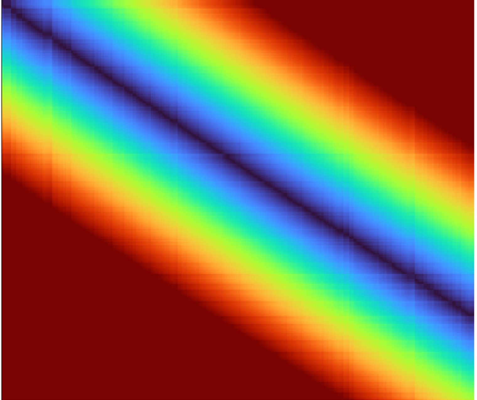
Figure 1 shows the absolute value of the residual arrival time ‘error’ in a plot of velocity versus ɛ, for the simple half-space model for a range of source-receiver offsets. To compute these errors, I first randomly perturbed the initial and density values, and then compared the computed arrival time for each perturbation to the ‘correct’ baseline arrival time for the starting model values of these elastic parameters. The plots show the absolute value of the difference (the ‘residual’) between the ‘ground truth’ baseline model arrival times and times from models with perturbed parameters. Hence, parameter combinations with very small residuals will give rise to measured data that are indistinguishable from each other (within some resolution criterion range). On this and all such subsequent figure, the cross-hairs indicate the associated baseline values.
The arrival time (denoted in Equation 12) at the reference offset is computed for anisotropic moveout calculated using the velocity defined in Equation 8 for the associated angle of incidence at the reflector. As can be seen in the figure, there is a range of values for which the arrival time error is near zero: in other words, any combination of velocity Vp and ɛ (within the tolerance of the resolution criterion) will produce the observed arrival time equally well. This region in the model space where the combinations of velocity and ɛ all describe the moveout behaviour equally well, can be thought of as being an approximate representation of the inversion null space or of a ‘region of ambiguity’. In other words, the parameters velocity and ɛ (and likewise δ) are not unique, and using them to characterise the rock physics will give rise to uncertainty in the results. As expected, for the shorter offsets where ɛ is not influential on the traveltimes, there is little interdependency between velocity and ɛ.
For the four offsets considered in Figure 1, we note that the region of the [Vp(0) ɛ] model space with small residual varies differently. For a more practical assessment representative of a real seismic experiment, in Figure 2 I show an average of the absolute residual error by combining the absolute value of residuals over a range of offsets; essentially, a superposition of individual residuals as shown in Figure 1, but now averaging over 501 offsets between 0 and 8000 m, with 501 perturbations of both Vp(0) and ɛ. Now the residual is more localised. On the left of the figure, is plotted the absolute traveltime error values averaged over the specified offset range, and in the centre, I have applied a resolution criterion (accepting combinations of [Vp ɛ] which give rise to traveltimes within ±2 ms of the baseline value), highlighting the region approximately representative of the model’s inversion ‘null space’ wherein lie the indistinguishable combinations of velocity and ɛ. Repeating the analysis for a less optimistic traveltime error tolerance by using the Rayleigh criterion of ¼ period (which is ~6.5 ms for a 30 Hz centre frequency), we get the results shown in Figure 2c, indicating a much larger region of ambiguity.
Repeating the analysis shown in Figure 2 for different maximum offset ranges highlights how, as expected, ɛ is not well constrained for small offsets. Table 3 shows the respective errors for a single offset and Table 4 shows the results for an average over a range of offsets (all using a minimum offset of 0 m), where the parameter baseline values were: Vp(0) = 2916 m/s, ɛ = 0.16). Results for absolute traveltime errors of 2 ms and also for the more pessimistic ¼ period tolerance (6.5 ms) for a 30 Hz Ricker wavelet are shown. Remember that for the majority of FWI iterations, the wavelet periods being considered are long, hence the larger tolerance results are perhaps more realistic.
Offset (m) |
| 4000 | 6000 | 8000 | 10000 |
dV (m/s) | ± | 3.6 | 3.13 | 2.72 | 2.47 |
dV (%) | ± | 0.12 | 0.11 | 0.09 | 0.08 |
Table 3. Velocity errors for absolute traveltime tolerance of 2 ms at baseline ɛ for the specified offset.
| For absolute traveltime tolerance of 2 ms. | |||||
| Maximum offset (m) | 4000 | 6000 | 8000 | 10000 | |
| dV (m/s) | ± | 6.11 | 6.77 | 7.54 | 8.14 |
| dV (%) | ± | 0.21 | 0.23 | 0.26 | 0.28 |
| dɛ | ± | 0.01 | 0.01 | 0.01 | 0.00 |
| dɛ (%) | ± | 7.70 | 3.74 | 2.89 | 2.62 |
| For traveltime tolerance of ¼ period (6.5 ms). | |||||
| Maximum offset (m) | 4000 | 6000 | 8000 | 10000 | |
| dV (m/s) | ± | 20.14 | 22.27 | 24.42 | 27.00 |
| dV (%) | ± | 0.69 | 0.76 | 0.84 | 0.93 |
| dɛ | ± | 0.04 | 0.02 | 0.02 | 0.01 |
| dɛ (%) | ± | 22.61 | 12.28 | 9.38 | 8.67 |
Table 4. Velocity and ɛ errors averaged over an offset range (with minimum offset = 0 m). For absolute traveltime tolerance of 2 ms.
The good news here is that velocity is well constrained in any analysis over a reasonable range of offsets, but unfortunately, ɛ is poorly constrained until we employ long offsets (as a well-known ‘rule of thumb’, we have good velocity resolution for ‘offset = target depth’, but for ɛ we need ‘offset = twice target depth’ for comparable resolution). It might seem counterintuitive that the velocity resolution error increases with offset, but this is due to the interaction with the simultaneous perturbation of ɛ. Looking at the spread of velocities within the tolerance band just at the reference value of ɛ (0.16) we do indeed note that increasing offset does reduce velocity error, as seen in Table 3.
A similar comparison for the variation of δ with ɛ is shown in Figure 3. For the 2 ms arrival-time tolerance, the errors are significant for δ, but for the 6.5 ms (¼ period at 30 Hz) criterion they are very large.
As with the above analysis for variation in traveltimes, we can also assess changes in amplitude behaviour. Consider the shale example just discussed, located on top of a sandstone layer. If we use values characteristic of sandstones (Ma et al. 2024) and using the anisotropic Zoeppritz equations to compute the amplitude of a reflection at the interface, we can use this value as a reference to compare to a suite of amplitude values obtained after randomly perturbing and density in the upper shale layer whilst keeping the elastic parameters constant in the lower, sandstone layer.
Whereas characterising the error for traveltimes was straightforward, for amplitude behaviour it is more complicated, as amplitudes can change radically over an offset range due to the underlying AVA response to the elastic parameters being used. For example, for a given maximum offset, changing the offset sampling can significantly change the result. This is because, as the reflections approach the critical angle, the amplitude of the reflection can increase drastically. So, decreasing the offset sampling, say from 100 m to 50 m, would change the error measurement, as finer sampling of the modelled data near the high amplitude critical angle events will bias the result (for a given constant offset sampling increment, the angular sampling increment will be smaller at larger offsets). This tends to make the error region smaller, due to the increased sensitivity to large amplitude changes. In other words, having good angular sampling near the critical angle can improve the inversion results by increasing sensitivity and reducing the error region. In the modelling conducted here, the offset range is 0-8 km with 101 traces (unless stated otherwise). Figure 4 shows the AVA response for the parameters being used, for anisotropic Knott-Zoeppritz modelling with Q = 100. As can be noted, a dense sampling near the critical angle will dominate the sensitivity to error.
Given the significant change in amplitudes with change in offset, x, here the norm characterising the error for parameters p1 and p2, is taken as the absolute value of the normalised residual, i.e.:
where the baseline value is the amplitude for the reference model at this offset, and this normalised residual error is then averaged across the offset range used. The traveltime norm was simply the absolute sum (over offsets) of residual traveltimes.
Figure 5a shows the relative amplitude error (as compared to the reference) plotted against variation in the associated velocity Vp(0) and ɛ, indicating the region of the model space for which we have an amplitude value within ±10% of the baseline value. In this case, these similar amplitudes could be obtained with velocity Vp(0) varying between about 2909 to 2922 m/s (i.e. within about ±0.2% of the baseline value of 2916 m/s) and ɛ varying between 0.14 to 0.19 (i.e. within about ±14% of the baseline value of 0.16). As with the traveltime errors, and as expected, velocity is better constrained than ɛ. For comparison, and to give an indication of a norm incorporating both time and amplitude errors, the black dashed-line overlay on Figure 5a shows the approximate null-space indicator from Figure 2c, highlighting the traveltime ambiguity area. Combining both traveltime and amplitude measurements into the FWI norm has the potential to reduce uncertainty in the inversion.
Figure 5b shows the relative amplitude error (as compared to the reference) plotted against variation in the associated velocity Vp(0) and Vs(0), indicating the region of this model space for which we have an amplitude value within ±10% of the baseline value. In this case, these similar amplitudes could be obtained with velocity Vp(0) varying between about 2909 to 2923 m/s (i.e. within about ±0.2% of the baseline value of 2916 m/s) and Vs(0) varying between 1644 to 1689 m/s (i.e. within about ±1% of the baseline value of 1669 m/s). Comparable analyses are shown for: c) Vp(0) versus density and d) Vs(0) versus density.
Figure 6 shows the effect of perturbing both Q and Vp(0) in the upper shale layer (i.e. Vp(0) via Equation 1, with traveltime dependence on angular velocity from Equation 12) for a range of values in the vicinity of the baseline model. Here the baseline Q values for the two examples shown were 20 and 100 with centre frequency 30 Hz, and in this case, the range of Vp(0) velocities for which the amplitude measurements would be similar is again about 10 m/s, whereas for the baseline Q = 100 case, Q has an uncertainty ranging from a lower value to about 95 up to the maximum value of 105 (i.e. within about ±5% of the baseline value). Repeating the analysis for small Q values results in a far smaller uncertainty, as small percentage changes in a low Q value will produce large amplitude changes and thus be more readily measurable and invertible.
Discussion
With a more complete theoretical description of wave propagation, now potentially including surface waves, guided waves, multiple reflections and elastic behaviour, in principle FWI can work with the complete recorded wavefield, thereby taking account of the underlying matrix parameters and density. Unfortunately, for the majority of seismic data available today, we do not have access to direct measurements of density or shear-wave velocity. Hence, any inversion based on such measured P-wave data will be trying to unpick the relationships between the and density parameters, along with anelastic Q effects. However, increasing use of the horizontal components in land and ocean bottom data will facilitate adoption of more complete implementations of elastic FWI, wherein the inversion can make use of the shear-related information directly.
Despite the limitations due to parameter interdependency discussed in this paper, given that we have a wide-range of offsets available from the seismic field data, individual traveltime errors on single offsets will be compensated for by other such measurements, and likewise, amplitude information from the range of available offsets will also help to constrain the inversion to enable robust estimation of the underlying elastic parameters from the AVA behaviour observed in the data. Having long offsets in the data increases diving-wave penetration and helps the inversion to update the velocity model using refractions. In addition, having these long offsets can also increase sampling in the vicinity of the critical angle, and thereby help to improve inversion using amplitude information. Although we might be fairly modest in only asking to update anisotropic Vp and P-impedance, using an elastic modelling engine facilitates better emulation of the P-wave behaviour and hence delivers more robust estimation of the P-wave parameters than can be obtained from a purely acoustic inversion scheme. In the modelling results presented here, for the Rayleigh ¼ period resolution criterion, parameter errors appeared to be acceptable. Additionally, as an FWI algorithm iterates, the overall reconciliation and volumetric balancing of errors will help convergence to acceptable model parameter estimates.
Unfortunately, but not surprisingly, FWI is still not a panacea, and will struggle with data that suffers from a large amount of near surface scattering due to small-scale heterogeneity. This is primarily because FWI is an indirect inversion scheme and as such, requires an initial model estimate to commence the parameter estimation procedure. If the starting model is too far from reality, then the iterative inversion procedure is unlikely to converge to an adequate model. In addition, very high frequencies would be needed to model (and invert for) such small-scale scattering effects, which would require small modelling cells (although adaptive grid methods such as an SE propagator can help overcome this limitation). Hence, for land data with severe near surface problems, FWI is still likely to struggle to converge to a reliable result. In addition, to ensure convergence to a reliable non-cycle-skipped FWI model, low frequencies (< 2 Hz) are usually required, and this in itself poses a challenge for contemporary acquisition methods.
Acknowledgements
I would like to thank Gary Margrave and the University of Calgary CREWES consortium for access to their isotropic MATLAB Zoeppritz modeller, and Ahmed Elbassiony, John Brittan, Carlos Calderón-Macías, Jaime Ramos-Martinez, Peter Rowbotham, Milad Farshad, Clement Kostov, and the anonymous reviewer for their careful proof reading and helpful suggestions which have improved the manuscript.
Appendix 1
Derivation of multi-parameter acoustic or elastic wave equations to facilitate FWI.
Wave equations take-on various forms. In their more complete forms, they derive from the Navier-Stokes equation after dropping mass-transport (‘material derivative’) terms (e.g. Pelissier et al., 2007). However, until very recently, the majority of the forms of the wave equation used in seismic data processing were based on an acoustic version, obtained after dropping the curl terms in the Navier-Stokes equation, thereby removing the shear terms, and often also assuming that density was either constant or coupled simply to velocity (e.g. Gardner et al., 1974).
As an aside, it is perhaps of interest to note that if we retained the mass-transport terms in the Navier-Stokes equation and dropped the Vp and Vs wave propagation terms, that we could then derive Darcy’s law for monitoring of reservoir fluids moving in a permeable medium (Pelissier et al., 2007).
Perhaps counterintuitively, even these acoustic forms of the wave equation could still be employed to deliver estimates of elastic parameters by analysing the amplitude behaviour of the data as a function of offset or angle (e.g. Connolly, 1999; Whitcombe et al., 2002). Recent examples of this approach in the context of acoustic waveform inversion are outlined in the works of Whitmore et al. (2020) and also McLeman et al. (2021) who both derive a form of the acoustic wave equation with a change of variables in order to solve for impedance as well as related elastic parameters, as well as for velocity. These forms have been promoted to furnish direct estimates of reflectivity (thereby obviating the need for a subsequent separate migration to obtain an image).
Starting from
for constant values of λ and μ, where is the particle displacement vector, ρ is the density, is the body-force vector, and λ and μ are the Lamé parameters defined in Equations 10 and 11, and noting that the compressional and shear velocities are given by:
we can write:
Applying the curl curl vector identity yields:
and rearranging gives:
In both A1.3 and A1.5, ignoring body forces and shear terms yields the two-way wave equation and for constant density the equations simplify to become the wave equation that was in industrial use for many years:
Used as a modelling engine in RTM and also in basic FWI implementations, this equation was in widespread use until very recently. The first step in improving it was to reintroduce a variable density term, and in the context of FWI, to extend the inversion from being from Vp only, to simultaneous inversion for Vp plus one other parameter such as ɛ or impedance, but still in the context of an acoustic formulation. More recently, a more complete elastic formulation has been adopted so as to produce more reliable inversion results for Vp, P-impedance, and shear-related parameters such as Vp/Vs, an example of which is shown later in this appendix.
In my previous FWI tutorial (Jones, 2019), I considered the case of inverting solely for velocity with a constant density assumption. In this case, the gradient (which describes the required model update) is computed by propagating two wavefields:
- a forward propagation of a source-term and taking its second time derivative at each propagation time-step and scaling with a term related to the derivative of the wave equation (with respect to velocity) and
- back propagating a residual (adjoint source term), related to the error between the modelled and observed data. This residual could be the simple difference between the observed and modelled data (thus pertaining to the dynamic amplitude differences), or perhaps be related to time shifts or phase differences between them (pertaining primarily to the kinematics).
If we wanted to expand the inversion to seek an update to a second parameter (such as P-wave anisotropic ɛ or P-impedance), then we would need to compute an associated gradient for this additional parameter. Doing this would not entail repeating the forward propagation of the source term and back propagation of the residual, but rather just computing new additional weighting terms to be applied at each time-propagation step. These weights would be related to the derivative of the wave equation with respect to the variable being updated.
In its simplest form with a constant density (equation A1.6), the wave equation can be solved straightforwardly for each of these two wavefields by dealing only with the strain relationships for velocity, and hence solving for a single uncoupled differential equation for each of the downgoing and upcoming wavefields.
As soon as we add complexity, such as for an elastic medium, we would then need to simultaneously solve a pair of differential equations (one related to stress and one to strain) for each of the propagation directions (similar to Equation A1.16 shown later).
Next, I will outline the formulation of one such approach for the multi-parameter joint inversion for Vp and P-wave impedance, Z, as presented by Whitmore et al. (2020) for the acoustic case, and thereafter briefly describe a more complete elastic modelling formulation. Whitmore et al. outline their approach starting from the isotropic acoustic wave equation and proceed to recast it in terms of impedance, rather than velocity and density. This sidesteps the usual problem of having to deal explicitly with density. Rather than starting from a wave equation expressed for particle displacement as is done in a similar multi-parameter inversion described by McLeman et al. (2021), Whitmore et al. commence with a version using pressure, P:
where: v is wave speed, ρ is density, and s is the source term.
Noting that impedance Z= ρ v, this can be rewritten to eliminate the explicit density terms, as:
This can be simplified so as to separate the velocity and impedance derivative terms, by twice using the divergence theorem product rule: recall that for scalar f and vector quantity k, we can write:
In the first step, equating and , the second LHS term in (A1.8) can be re-written giving:
In the second step, equating f = v and , and decomposing the 2nd LHS term, this becomes:
As the impedance is a scalar field, the gradient of its inverse can be rewritten as follows:
Substituting this into the third LHS term in (A1.11) yields:
Rearranging as per Whitmore et al. yields:
Noting that the term represents the impedance change with direction (the vector reflectivity), they then introduce R to represent this term:
So, in principle, the reflectivity as a function of direction (reflection angle) can be computed as part of the numerical solution of equation A1.15. This approach is analogous to the Poynting-vector implementation of RTM, wherein using a tau-p transform we partition the shot into angle classes at every propagation step so as to facilitate direct output of angle gathers from the migration. Examples in the context of FWI can be found in Jin et al. (2020, 2024).
Extending the modelling to become elastic
For a more complete approach to the forward modelling, an elastic equation can be used, incorporating an explicit term for Vs, by essentially reintroducing the curl-related term dropped in equation A1.6. However, the majority of available measured data are either recorded on hydrophones in the marine case or use only the vertical geophones on land or at the seabed. Consequently, we need to either: - use a functional relationship between Vp and Vs, calibrated against any available well-logs; or, estimate shear terms by assessing the AVA behaviour in the P-wave data; or, rely on somehow exploiting S-wave energy that has been converted to P-waves in the recordings (as is described by Li and Wu, 2020).
Alternatively, the modelling equations can be cast in terms of the , although the inversion might only be seeking to update the combination of them that define Vp. This approach is taken by Macesanu et al. (2024) and likewise by Huang et al. (2025).
Starting from an elastic wave equation, separating dynamic (stress and strain) terms from the kinematic (velocity) terms, Macesanu et al. have:
where is the stress matrix is the velocity, and is a source-related term.
We now have two differential equations that need to be solved simultaneously. Unfortunately, each one requires the results of the other in order to be solved. One way of achieving this is to employ the staggered time grid approach (Virieux 1984) where we first propagate one of the equations over a time step, and use its output to plug into the other and then solve the second equation using the values just obtained from the solution of the first. The grids for the two propagations are usually shifted by half a grid so as to help mitigate the effects of numerical dispersion.
Perhaps counterintuitively, formulating an elastic modelling algorithm is not that difficult: in fact, it is anisotropic modelling that poses most algorithmic difficulty, as we have to deal with velocity that changes as a function of wave propagation direction. As noted earlier, in the section on elastic and anisotropic behaviour, the difficulties with elastic modelling can be summarized as follows:
- ideally, we should estimate a starting value for Vs by performing Vs velocity analysis on measured field data, and also inverting against actual field data measurements for the shear parameters, but this can only be done if we actually recorded horizontal components of the wavefield. Most often, we are working with only compressional wave data (from pressure or vertical component measurements) hence do not have direct access to Vs.
- needing reasonable estimates of both density and Vs in order to commence the modelling. Although we can use a modified Gardner relationship to obtain a density proxy, this only holds for clastic sediments, and for Vs although we can take Vs as being about half Vp, for some near surface materials Vs can be as low as a few tens of m/s, so using Vs = Vp/2 is then highly inaccurate.
- the cost of modelling shear waves is much greater than modelling compressional waves. The difficulties in dealing with very low near-surface velocities can be mitigated to some extent by using an adaptive modelling grid, using small cells in the low velocity regions and much larger cells elsewhere.
Consequently, we can see that both elastic modelling and FWI are indeed achievable but that we need to be fully aware of the assumptions and approximations being made in order to have a good grasp of how reliable the obtained results are likely to be.
References
- Aki, K. and Richards, P.G. [1980] Quantitative Seismology, theory and methods. Freeman, 932 pages.
- Aktharuzzaman, M. [2024] Full Waveform Inversion-Based Ultrasound Computed Tomography for Material Characterization. University of Alabama Libraries. https://ir.ua.edu/handle/123456789/15347.
- Carroll, N.L., Humphrey, V.F., and Smith, J.D. [2002] Energy and phase velocity considerations required for attenuation and velocity measurements of anisotropic composites. Ultrasonics, 40, 525-530.
- Chemingui, N., Yang Y., Ramos-Martinez, J., Huang, G., Whitmore, D., Crawley, S., Klochikhina, E., and Arasanipalai, S. [2023] Simultaneous inversion of velocity and angle-dependent reflectivity. SEG Annual Meeting, Expanded Abstracts.
- Connolly, P. [1999] Elastic impedance. The Leading Edge, 18, 438-452.
- Domnesteanu, P.R., Domnesteanu, R., and McCann, C. [2001] The anisotropic response of shale elastic stiffness coefficients to overpressure. 71st SEG Annual International Meeting, Expanded Abstracts.
- Futterman, W.I. [1962] Dispersive Body Waves. Journal of Geophysical Research, 67(13), 5279-5291.
- Gardner, G.H.F., Gardner, L.W., and Gregory, A.R. [1974] Formation Velocity and Density – The Diagnostic Basics for Stratigraphic Traps. Geophysics, 39, 770-780.
- Guash, L., Agudo, O.C., Tang, M.X., Nachey, P., and Warner, M. [2020] Full-waveform inversion imaging of the human brain. NPJ Digit. Med., 3, 28.
- Haacke, R., Riley-Watson, A., Grimshaw, C., Dobo, Z., King, A., Knapp, S., Schiott, C., Vejbaek, O., Rosengreen, M., and Hidalgo, C. [2019] Practical Multi-Parameter FWI at the South Arne Field. 81st EAGE Annual Conference and Exhibition, Extended Abstracts.
- Huang, Y., Mao, J., Sheng, J., Perz, M., He, Y., Hao, F., Liu, F., Wang, B., Yong, S.L., Chaikin, D., Citlali-Ramirez, A., Hart, M., and Roende, H. [2023] Toward high-fidelity imaging: Dynamic matching FWI and its applications. The Leading Edge, 42, 124-132.
- Huang, G., Macesanu, C., Liu, F., Ramos-Martinez, J., Whitmore, D., Calderon, C., and Bloor, R. [2025] Multiparameter elastic FWI for joint inversion of velocity and reflectivity. 86th EAGE Annual Conference and Exhibition, Extended Abstracts.
- Jackson, D.D. [1972] Interpretation of inaccurate, insufficient, and inconsistent data. Geophysical Journal of the Royal Astronomical Society, 28, 97-109.
- Jiao, K., Sun, D., Cheng, X., and Vigh, D. [2015] Adjustive full waveform inversion. 85th SEG Annual International Meeting, Expanded Abstracts, 1091–1095.
- Jin, H., Vu, P., Liao, Q., Zhou Y., and Chu, C. [2020] 3D RTM sparse angle gathers. 90th SEG Annual International Meeting, Expanded Abstracts.
- Jin, H., Luo, S., Liao, Q., Shen, X., Xia, G., Vyas, M., Williams, C. [2024] FWI derived reflectivity angle gathers. 85th EAGE Annual Conference and Exhibition, Extended Abstracts.
- Jones, I.F. [2018] Velocities, Imaging, and Waveform Inversion (The evolution of characterizing the Earth’s subsurface). EAGE, EET 13, 234 pages.
- Jones, I.F. [2019] Tutorial: The mechanics of waveform inversion. First Break, 37(5), 31-43.
- Jones, I.F, Felicio, R., Vlassopoulou, A., and Hagen, C. [2019] Tutorial: tomographic Bayesian uncertainty estimation. First Break, 37(9), 37-48.
- Jones, I.F., Calderon-Macias, C. Ong, B., and Berranger, I. [2023] Tutorial: least squares migration and full waveform imaging. First Break, 41(3), 27-35.
- Knott, C.G. [1899] Reflexion and refraction of seismic waves with seismological applications. Transactions of the Seismological Society of Japan. Reprinted in: Pelissier, et al., 2007.
- Lailly, P. [1983] The seismic inverse problem as a sequence of before stack migrations. Conference on inverse scattering: Theory and application, SIAM, 206-220.
- Li, Q. and· Wu, G. [2020] 2D multi-parameter waveform inversion of land reflection seismic data obtained from the particle-motion response from the vertical geophone. Acta Geophysica, 68, 377-388.
- Liu, J., Yang, M., Deeds, J., Luckow, J., Cheriyan, T., Ariston, P-O., Yang, Z., Mei, M., and Zhang, Z. [2021] Solving subsalt imaging challenges in Green Canyon using OBN and FWI Imaging. 91st SEG Annual International Meeting, Expanded Abstracts.
- Love, A.E.H. [1927] A treatise on the mathematical theory of elasticity. Dover, New York, 4th Edition. 643 pages.
- Ma, Z.Q., Yin, X.Y., Zong, Z.Y., Tan, Y.Y., and Yang, Y.M. [2024] Analytical solution for the effective elastic properties of rocks with the tilted penny-shaped cracks in the transversely isotropic background. Petroleum Science, 21, 221-243.
- Macesanu, C., Liu, F., Huang, Y., Mao, H., and Calderon, C. [2024] Implementation aspects of elastic FWI and its application to sparse OBN data. SEG: Fourth International Meeting for Applied Geoscience and Energy, Expanded Abstracts, 886-890.
- Maharramov, M., Baumstein, A.I., Tang, Y., Routh, P.S., Lee, S., and Lazaratos, S.K. [2017] Time-domain broadband phase-only full-waveform inversion with implicit shaping. SEG Technical Program, Expanded Abstracts, 1297-1301.
- Mao, J., Sheng, J., Huang, Y., Hao, F., and Liu, F. [2020] Multi-channel dynamic matching full-waveform inversion. 90th SEG Annual International Meeting, Expanded Abstracts, 666-670.
- Mavko, G., Mukerji, T., and Dvorkin, J. [1998] The Rock Physics Handbook. Cambridge University Press. Pp329.
- Mavko, G. and Jizba, D. [1991] Estimating grain-scale fluid effects on velocity dispersion in rocks. Geophysics, 56, 1940-1949.
- McLeman, J., Burgess, T., Sinha, M., Hampson, G., and Thompson, T. [2021] Reflection FWI with an augmented wave equation and quasi-Newton adaptive gradient scheme. SEG/AAPG First International Meeting for Applied Geoscience & Energy, Expanded Abstracts, 667-671.
- McLeman, J., Burgess, T., and Rayment, T. [2022] FWI imaging with simultaneous anisotropy estimation: 83rd EAGE Annual Conference and Exhibition, Extended Abstracts.
- Menke, W. [1989] Geophysical Data Analysis: Discrete Inverse Theory, Revised Edition. International Geophysics Series, 45. Academic Press, Inc.
- Métivier, L., Brossier, R., Mérigot, Q. Oudet, E., and Virieux, J. [2016a] Measuring the misfit between seismograms using an optimal transport distance: Application to full waveform inversion. Geophysical Journal International, 205(1), 345–377.
- Métivier, L., Brossier, R., Mérigot, Q., Oudet, E., and Virieux, J. [2016b] Increasing the robustness and applicability of full wave-form inversion: an optimal transport distance strategy. The Leading Edge, 35, 1060-1067.
- Mora, P. [1988] Elastic wavefield inversion of reflection and transmission data. Geophysics, 53, 750-759.
- Osypov, K., Nichols, D., Woodward, M., Zdraveva O., and Yarman, C.E. [2008] Uncertainty and resolution analysis for anisotropic tomography using iterative eigendecomposition. 78th SEG Annual Meeting, Expanded Abstracts.
- Osypov, K., Yang, Y., Fournier, A., Ivanova, N., Bachrach, R., Yarman, C.E., You, Y., Nichols, D., and Woodward, M. [2013] Model-uncertainty quantification in seismic tomography: method and Applications. Geophysical Prospecting, 61, 1114-1134.
- Pavlopoulou, P. and Jones, I.F. [2020] The influence of source wavelet-estimation error in acoustic time domain full waveform inversion. First Break, 38(7), 33-38.
- Pelissier, M.A., Hoeber, H., van de Coevering, N., and Jones, I.F. [2007] Classics of Elastic Wave Theory. SEG Geophysics Reprints, 24, Series Editor: Daniel A. Ebrom, 534 pages.
- Plessix, R.-E. [2006] A review of the adjoint-state method for computing the gradient of a functional with geophysical applications. Geophysical Journal International, 167(2), 495-503.
- Plessix, R.-E. [2007] A Helmholtz iterative solver for 3-D seismic-imaging problems. Geophysics, 72, SM185-194.
- Pratt, R.G., Song, Z.M., Williamson, P., and Warner, M. [1996] Two-dimensional velocity models from wide-angle seismic data by wavefield inversion. Geophysical Journal International, 124, 323-340.
- Pratt, R.G. [1999] Seismic waveform inversion in the frequency domain, Part 1: theory and verification in a physical scale model. Geophysics, 64, p. 888-901.
- Pratt, R.G. and Shipp, R.M. [1999] Seismic waveform inversion in the frequency domain, Part 2: Fault delineation in sediments using crosshole data. Geophysics, 64, 902-914.
- Ramos-Martinez, J., Crawley, S., Zou, Z., Valenciano, A., Klochikhina, E., and Chemingui, N. [2016] A robust FWI gradient for high-resolution velocity model building. 87th SEG Annual International Meeting, Expanded Abstracts, 1258-1262.
- Rayment, T., Dancer, K., McLeman, J., and Burgess, T. [2022b] High-resolution FWI imaging — An alternative to conventional processing. 83rd EAGE Annual Conference and Exhibition, Extended Abstracts.
- Rayment, T., McLeman, J., Dancer, K., and Burgess, T. [2022a] Next-generation resolution through multiparameter FWI imaging. SEG/AAPG Second International Meeting for Applied Geoscience & Energy, Expanded Abstracts, 922-926.
- Ruger, A. [2001] Reflection coefficients and azimuthal AVO analysis in anisotropic media. Geophysical Monograph Series, 10, 189 pages.
- Salaun, N., Reinier, M., Espin, I., and Gigou, G. [2021] FWI velocity and imaging: A case study in the Johan Castberg area. 82nd EAGE Annual Conference and Exhibition, Extended Abstracts.
- Sayers, C.M. and den Boer, L.D. [2018] The Elastic Properties of Clay in Shales. Journal of Geophysical Research. Solid Earth, 123, 5965-5974.
- Schuster, G.T. [1993] Decomposition of the waveform gradient into short and long wavelength components. Annual Report of the Utah Tomography and Modelling/Migration Consortium, 79-88.
- Schuster, G.T. [2017] Seismic Inversion. Investigations in Geophysics, 20.
- Sirgue, L. and Pratt, R.G. [2004] Efficient waveform inversion and imaging: a strategy for selecting temporal frequencies. Geophysics, 69, 231-248.
- Svitek, T., Vavrycuk, V., Lokajicek, T., and Petruzalek, M. [2014] Determination of elastic anisotropy of rocks from P- and S-wave velocities: numerical modelling and lab measurements. Geophys. J. Int., 199, 1682-1697.
- Symes, W.W. [2008] Migration velocity analysis and waveform inversion. Geophysical Prospecting, 56, 765-790.
- Tarantola, A. [1984] Inversion of Seismic Reflection Data in the Acoustic Approximation. Geophysics, 49, 1259-1266.
- Tarantola, A. [1987] Inverse problem theory. Elsevier.
- Tarantola, A. [1988] Theoretical background for the inversion of seismic waveforms, including elasticity and attenuation. Pure and Applied Geophysics, 128(1–2), 365-399.
- Thomsen, L. [1986] Weak elastic anisotropy. Geophysics, 51, 1954-1966.
- Thomsen, L. [1993] Weak anisotropic reflections. In: Castagna, J.P., and Backus, M. Offset-dependent reflectivity—Theory and practice of AVO analysis. Soc. Expl. Geophys., p. 103-111.
- Tromp, J. [2020] Seismic wavefield imaging of Earth’s interior across scales. Nature Reviews Earth & Environment, 1, 40-53.
- Vernik, L. and Liu, X. [1997] Velocity anisotropy in shales: A petrophysical study. Geophysics, 62, 521-532.
- Vigh, D., and Starr, E.W. [2008] 3D prestack plane-wave, full-waveform inversion. Geophysics, 73(5), VE135–VE144.
- Vigh, D., Jiao, K., Cheng, X., Sun, D., and Zhang, L.X. [2017] Seeing below the diving wave penetration with full waveform inversion. 87th SEG Annual International Meeting, Expanded Abstracts, 1466-1470.
- Virieux, J. [1984] SH-wave propagation in heterogeneous media: Velocity-stress finite-difference method. Geophysics, 49, 1933-1957.
- Virieux, J. and Operto, S. [2009] An overview of full-waveform inversion in exploration geophysics. Geophysics, 74, WCC1-WCC26.
- Virieux, J., Asnaashari, A. Brossier, R. Métivier, L., Ribodetti, A., and Zhou, W. [2017] An introduction to full waveform inversion. Chapter in: Encyclopedia of Exploration Geophysics. SEG, pp. R1-1-R1-40. Editors: Vladimir Grechka and Kees Wapenaar.
- Wang, Y. [2008] Seismic inverse Q filtering. Blackwell, ISBN 978-1-4051-8540-0, 249 pages.
- Wang, C., Delome, H., Calderon, C., Yingst, D., Leveille, J., Bloor, R., and Farmer, P. [2011] Practical strategies for waveform inversion. 81st SEG Annual International Meeting, Expanded Abstracts, 2534-2538.
- Wang, C., Farmer, P., Yingst, D., Jones, I., Calderon, C., and Brittan, J. [2018] Traveltime based reflection full waveform inversion. 80th EAGE Annual Conference & Exhibition, Extended Abstracts, Workshop 1.
- Wang, B., He, Y., Mao, J., Liu, F., Hao, F., Huang, Y., Perz, M., and Michell, S. [2021] Inversion-based imaging: From LSRTM to FWI imaging. First Break, 39(12), 85-93.
- Warner, M., Umpleby, A., Stekl, I., and Morgan, J. [2010] 3D full-wavefield tomography: imaging beneath heterogeneous overburden. 72nd EAGE Annual Conference & Exhibition, Extended Abstracts, Workshop 6.
- Warner, M.R. and Guasch, L. [2014a] Adaptive waveform inversion: Theory. 76th EAGE Annual Conference and Exhibition, Extended Abstracts.
- Warner, M.R. and Guasch, L. [2014b] Adaptive waveform inversion. 84th SEG Annual International Meeting, Expanded Abstracts, 1089-1093.
- Warner, M.R. and Guasch, L. [2015] Robust adaptive waveform inversion. 85th SEG Annual International Meeting, Expanded Abstracts, 1059-1063.
- Warner, M.R. and Guasch, L. [2016] Adaptive waveform inversion: Theory. Geophysics, 81(6), R429- R445.
- Whitcombe, D.N., Connolly, P.A., Reagan, R.L., and Redshaw, T.C. [2002] Extended elastic impedance for fluid and lithology prediction. Geophysics, 67(1), 63-67.
- Whitmore, N.D., Ramos-Martinez, J., Yang, Y., and Valenciano, A.A. [2020] Full wave field modeling with vector-reflectivity. 82nd EAGE Annual Conference & Exhibition, Extended Abstracts.
- Worthington, M.H. [1984] An introduction to geophysical tomography. First Break, 2, 20-26.
- Yang, Y. and Engquist, B. [2018] Analysis of optimal transport and related misfit functions in full-waveform inversion. Geophysics, 83 (1), A7-A12.
- Yang, Y., Ramos-Martinez, J., Whitmore, D., Valenciano, A.A., and Chemingui, N. [2020] Full Waveform Inversion Using Wave Equation Reflectivity Modeling. 82nd EAGE Annual Conference & Exhibition, Extended Abstracts.
- Yingst, D., Wang, C., Park, J., Bloor, R., Leveille, J.P., and Farmer, P. [2011] Application of time domain and single-frequency waveform inversion to real data. 73rd EAGE Annual Conference and Exhibition, Extended Abstracts.
- Zener, C. [1948] Elasticity and anelasticity of Metals. University of Chicago Press, Chicago.
- Zhang, Z., Wu, Z., Wei, Z., Mei, J., Huang, R., and Wang, P. [2020] FWI Imaging: Full-wavefield imaging through full-waveform inversion. SEG Technical Program, Expanded Abstracts, 656–660.
- Zoeppritz, K. [1914] On the reflection and transmission of seismic waves at surfaces of discontinuity. Transactions of the Royal Society of Sciences and Humanities, Gottingen. Translated in: Pelissier, et al., 2007.

